Monday Morning Mulling: December Challenge

On the final Friday of each month, set an Excel for you to puzzle over for the weekend. On the Monday, we publish a solution. If you think there is an alternative answer, feel free to email us. We’ll feel free to ignore you.

Final Friday Fix: December Challenge Recap

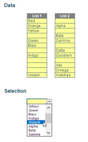
December’s challenge was another deceptively simple question. All you needed to do was to create an in-cell list that provided only non-blank choices from two columns of data, e.g.

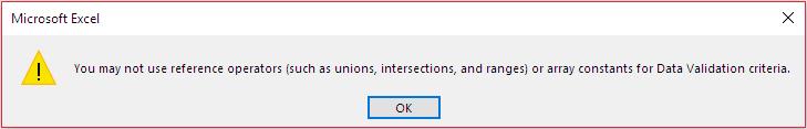
Forgetting the need to ignore blanks, there is another issue you may have encountered:

But let’s back up…

The Solution

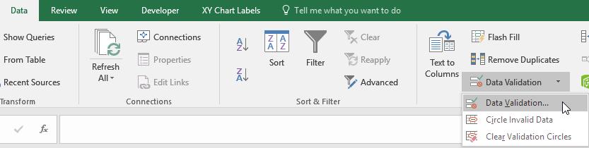
Given our challenge specifically stated that VBA or “anything that appears on the ‘Developer’ tab on the Ribbon” should not be used (e.g. combo boxes), this really restricted us to creating a list using Excel’s Data Validation feature. We have discussed Data Validation before (please refer to >Controlling Your Inputs). However, here’s the executive summary. By default, you can type anything into any cell in Excel, but you can restrict cell contents to “valid” data entries. This is the concept of data validation and Excel’s Data Validation feature. To access Data Validation, it can be found in the ‘Data Tools’ grouping on the ‘Data’ tab of the Ribbon:

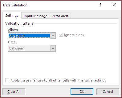
It’s probably easier to use the old Excel 2003 keyboard shortcut (ALT + D + L), although the Excel 2007 keyboard shortcut ALT + A + V + V works too. This displays the ‘Data Validation’ dialog box, which by default allows “Any value” to be contained within the selected cell(s):

This can be changed by changing the selection in the ‘Allow:’ drop down box. It may be modified to any of the following:

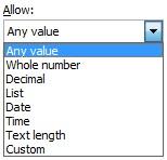
Most of these criteria do exactly what they say on the tin: by choosing ‘Decimal’, the input must be a number, whereas ‘Whole Number’ allows for integers only, etc. However, it is ‘List’ that we will focus on here, as this creates an in-cell drop-down box:

With ‘List’ selected, the dialog box prompts for a source for the list.

In the illustration, the entries have been typed in, separated by a comma. However, the data can use cell references which are in a column – or a row – as long as the cells are on the same worksheet. This can be limiting and a viable workaround is to name a range instead (see Naming Names for more details). For lists, we also strongly recommend using the ‘In-cell dropdown’ which provides a dropdown list of valid entries once the cell has been selected.

There are tricks you can employ to make the list source more flexible, typically using the INDIRECT function (please see Being Direct About INDIRECT for more details), but that won’t help you here. No matter how you try to combine your two lists, you are likely to receive the following error message:

So how do you get around this? Well, you have to go for a less elegant solution – and essentially build a list in one location (column or row) only. Our suggested solution uses the following attached Excel file.

Let’s start by specifying our example, viz.

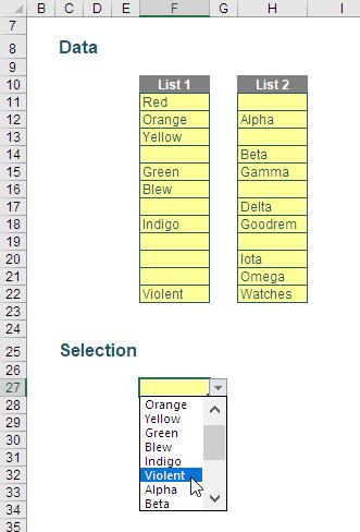
Cells F11:F22 have been named List1 and cells H11:H22 have been called List2 (surprise, surprise).

Next, I am going to add some “helper” calculations as follows:

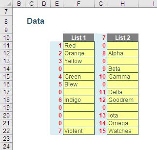
• The formula in cell E11 is

• This adds one to the running total starting in blank cell E10 if and only if the corresponding cell in column F is not blank (COUNTA essentially counts the number of non-blank cells in a range). This formula is copied down the column and the range has been named ListCounter01

• A similar formula is copied into cells G11:G22:

• This range has been named ListCounter02

• This just leaves cell G10:

• which takes the maximum figure from column E, so a “true” running total is computed. This cell has been named Max_List1.

• (These formulae have been hidden in the attached Excel file by using “;;;” custom number formatting. For more details on how this works, and number formatting in general, please refer to Knowing When Your Number’s Up.)

Next, some interim calculations were created:

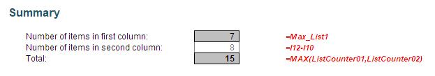
These three values (7, 8 and 15) were named First_Column_Count, Second_Column_Count and Total_Count respectively. These values are required as follows:

• Total_Count calculates how many items there will be in the amalgamated list to be generated
• First_Column_Count determines whether the item number in the list should come from List1 (if the record number is less than or equal to 7) or List2 (if the record number is between 8 and the Total_Count, 15)
• Second_Column_Count is created for completeness – and in case there is a third list of data at a later point in time.

A single list may now be generated (we strongly recommend keeping all your list data / lookup references on one sheet so they may be located quickly in larger spreadsheets):

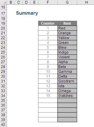
The formula in cell F20 is

This simply creates a counter running from 1 to Total_Count.

The formula in cell G20 is a little more sophisticated:

This uses the function combination INDEX MATCH (see >Are Things LOOKing UP for INDEX and MATCH? for more details) to reference the next non-blank entry in List1 and, once this has been exhausted, List2.

It’s easy from here. The data validated list may simply reference cells G20:G39 on this worksheet (called Calculations), or if you want to get more sophisticated, you can exclude the blank entries in the range (cells G35:G39) by defining what is known as a dynamic range name using the formula

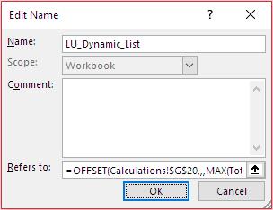
You can find out more about the OFFSET function and creating dynamic ranges in our article The Onset of OFFSET.

Assuming you have used this method and named the range LU_Dynamic_List, all that needs to be now is complete the definition of the data validated list, viz.

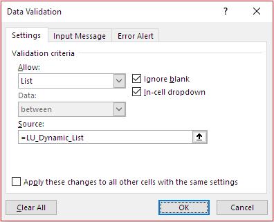
Nothing to it – except have a rudimentary understanding of Data Validation, COUNTA, MAX, range names, INDEX, MATCH and OFFSET! That’s why we liked this question!

The Final Friday Fix will return on Friday 26 January with a new Excel Challenge. In the meantime, please look out for the Daily Excel Tip on our home page and watch out for a new blog every other business workday.