Monday Morning Mulling: June 2025 Challenge

On the final Friday of each month, we set an Excel / Power Pivot / Power Query / Power BI problem for you to puzzle over for the weekend.  On the Monday, we publish a solution.  If you think there is an alternative answer, feel free to email us.  We’ll feel free to ignore you.

The Challenge

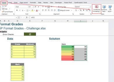
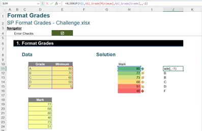
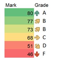
Last Friday’s challenge involved creating a set of grades, formatting and icons based upon a list of student marks.  The following example was provided:

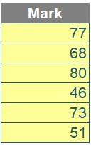
The single-column dataset Mark contained a list of marks.  Your challenge was to assign the correct background colour, icon and grade according to the tbl_Grade table, as shown in the dataset at the bottom.

You could download the original question file here.

The requirements were as follows:

• the formatting must be dynamic, meaning it should update automatically if the marks were to change
• you cannot use VBA, Office Scripts or any other programming code.

Suggested Solution

You can find our Excel file here, which shows our suggested solution.  The steps are detailed below.

This Final Friday Fix sounded simple (that’s because it is compared to some of our other ones!).  However, as you might have already realised, finding the right feature within Excel to complete even simple tasks can sometimes be tricky.

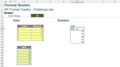
First, let’s sort the Mark column from the highest to the lowest.  Type the following formula into the cell, which sorts the values in our example file in cells D18:D23 in descending order, with ‘-1’ specifically indicating the descending sort of direction:

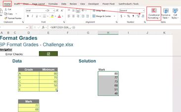
Then, let’s add a background conditional formatting to the Mark column, according to their marks.  Start by selecting the entire Mark column.  Then, go to the Home tab on the Excel Ribbon and click on ‘Conditional Formatting’ within the Styles group. 

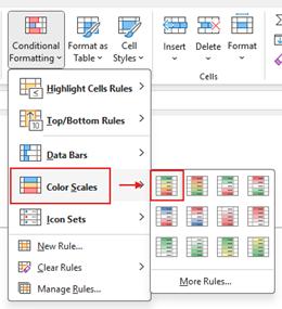
From the dropdown menu, choose ‘Color Scales’, and select the first option in the top row (pictured below).  This will automatically apply our gradient colour scale.

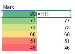
Next, to prepare for applying directional icon sets, type the formula to create a new column equals the value in the Mark  column.  Make sure to apply it to the rest of the rows.

Select the entire column we just created.  Then, go to the Home tab on the Excel Ribbon and click on ‘Conditional Formatting’ within the Styles group.

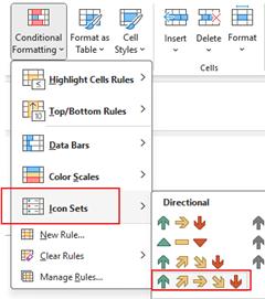
From the dropdown menu, choose ‘Icon Sets’, then select the five-arrow style under the Directional category (again, pictured).

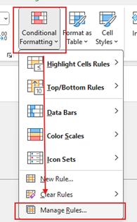
The column currently shows both an icon on the left and a mark on the right, with the icon based upon default percentage thresholds.  To display only the icons and apply a custom grade-based rule, go to the Home tab, click ‘Conditional Formatting’ in the Styles group, then select ‘Manage Rules…’.

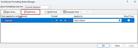
In the ‘Conditional Formatting Rules Manager’ dialog, click the ‘Icon Set’ rule then click ‘Edit Rule…’ to modify it. 

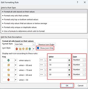
In the ‘Edit Formatting Rule’ dialog, check the ‘Show Icon Only’ box.  Then, set the Type to Number and adjust the values according to the grade ranges defined in the tbl_Grade table.  Click OK to apply the changes.

Next, we’ll add another column to assign a grade based on each student’s mark.

In this new column, we’ll use the XLOOKUP function to find the appropriate grade for each mark.  If you're new to XLOOKUP, it’s a powerful Excel function that searches a value in one column (in this case, the Minimum) and returns the corresponding value from another column (the Mark).  You can learn more about how XLOOKUP works in our detailed blog post here.

The formula we used is:

The fifth argument, ‘-1’, is called ‘match_mode’.  This tells Excel to perform an approximate match by finding the next smaller item if an exact match isn’t found.  This type of approximate match is ideal for descending grade scales and applies the grade based on the lower bound of the grade range.

To make the icons and grades appear as if they're in the same column, select the entire column and drag its edge to narrow the width.

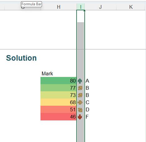
And this completes the process, giving us the final table with colour-coded marks, directional icons, and assigned grades—all neatly organised for easy interpretation.

We appreciate there are many, many ways this could have been achieved.  If you have produced an alternative, radically different approach, congratulations – that’s half the fun of Excel!

The Final Friday Fix will return on Friday 25 July 2025 with a new Excel Challenge.  In the meantime, please look out for the Daily Excel Tip on our home page and watch out for a new blog every business working day.