
Monday Morning Mulling: February 2024 Challenge
26 February 2024
On the final Friday of each month, set an Excel for you to puzzle over for the weekend. On the Monday, we publish one suggested solution. No-one is stating this is the best approach, it’s just the one we selected. If you don’t like it, lump it – or contact us with your preferred solution.
The Challenge
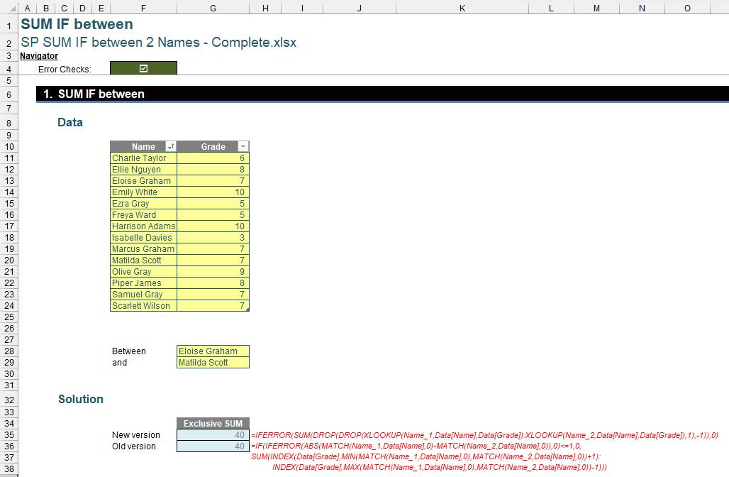
On Friday, we asked you to imagine you had a Table named Data in Excel, containing a list of names under the column Name and corresponding numerical data under the column Grade as follows:
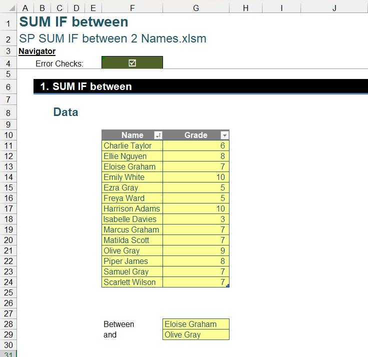
Your task was to write a single Excel formula that summed the Grade data between two [2] names exclusively, which we referred to as Name_1 (Cell G28) and Name_2 (Cell G29). These names were inputs that could be changed, and the sum was to dynamically update to reflect the range of data between these two [2] names in the Data table. You could download the original question filehere.
As always, there were some requirements:
- the formula needs to be within just one [1] column (no “helper” cells)
- the solution must work even if the order of Name_1 and Name_2 is swapped in the list
- the formula should be dynamic so that it updates when a new entry is added.
Suggested Solution for Modern Excel Users (Excel 365 and Later Versions)
You can find our Excel file here, which shows our suggested solution. The steps are detailed below.
Crafting a Data Range with XLOOKUP and Colon
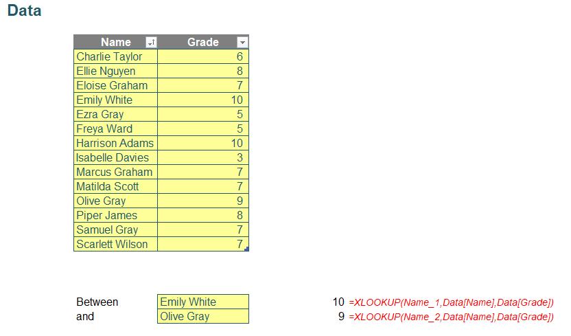
We begin our formula with the XLOOKUP function, deploying it twice to accurately retrieve the grades corresponding to Name_1 and Name_2.
=XLOOKUP(Name_1,Data[Name],Data[Grade])
=XLOOKUP(Name_2,Data[Name],Data[Grade])
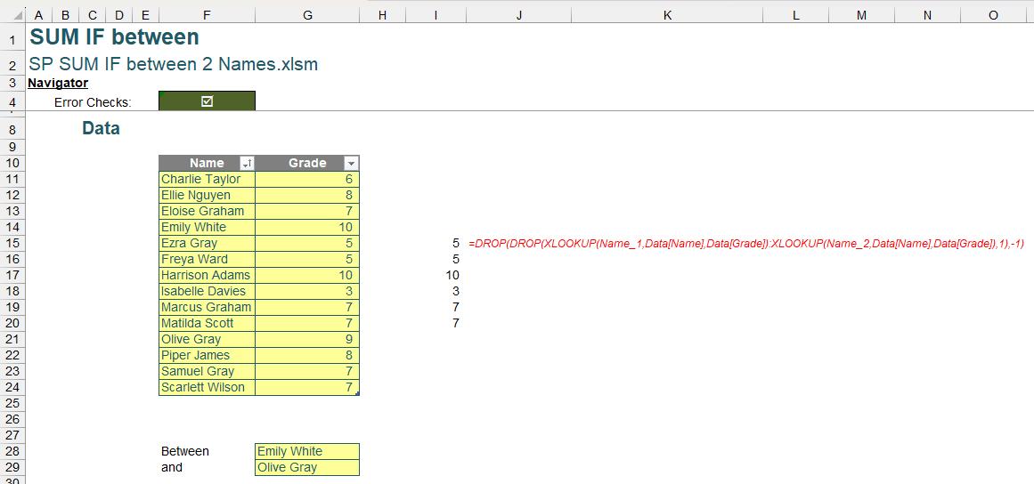
This will return us the respective grades for Name_1 and Name_2:
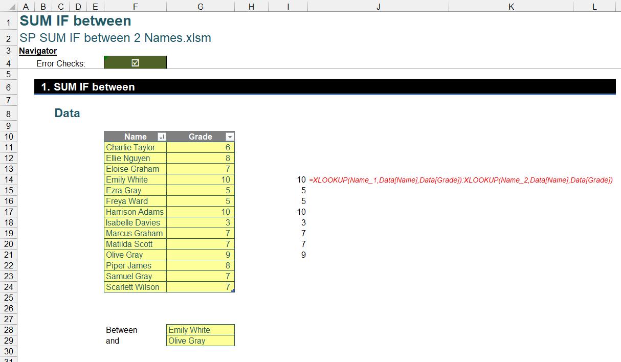
The real magic happens when we introduce a colon ‘:’ between these two [2] XLOOKUP functions. This action forms a dynamic array that spans from the grade of Name_1 to that of Name_2.
=XLOOKUP(Name_1,Data[Name],Data[Grade]):XLOOKUP(Name_2,Data[Name],Data[Grade])
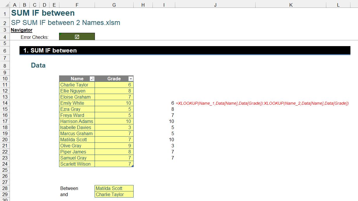
Even if the names selected from the dropdown are not in sequential order, this formula dynamically adjusts, ensuring the correct range is captured:
Refining the Range with DROP
At this stage, while we could directly sum the array and then subtract the two [2] values of the lookup, we opt for a more refined approach by incorporating the DROP function. This function is instrumental in sculpting our dynamic range further before performing the summation.
We can use:
=DROP(Range,1)
and
=DROP(Range,-1)
to remove the first and last entries in our range, the grades directly associated with Name_1 and Name_2.
Let’s combine all of that in this formula:
=DROP(DROP(Range,1),-1)
This formula removes the first and last row of our Range. When we substitute Range with our earlier XLOOKUP array, this returns the exact range we wish to sum:
=DROP(DROP(XLOOKUP(Name_1,Data[Name],Data[Grade]):XLOOKUP(Name_2,Data[Name],Data[Grade]),1),-1)
SUM and Error Trapping
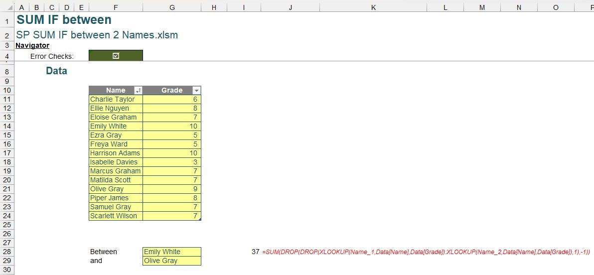
The penultimate step here is to SUM, hence we quickly add the SUM function here:
=SUM(DROP(DROP(XLOOKUP(Name_1,Data[Name],Data[Grade]):XLOOKUP(Name_2,Data[Name],Data[Grade]),1),-1))
However, we must consider edge cases, such as the non-selection of names or the selection of adjacent names, which could lead to errors in our formula:
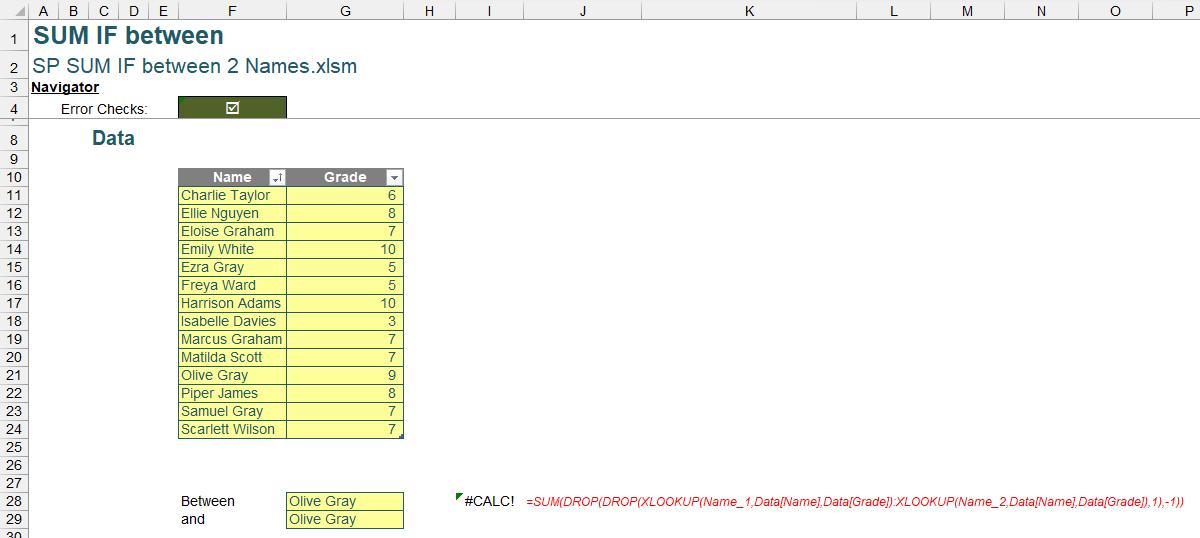
To address this, we wrap our summation formula within an IFERROR statement.
=IFERROR(SUM(DROP(DROP(XLOOKUP(Name_1,Data[Name],Data[Grade]):XLOOKUP(Name_2,Data[Name],Data[Grade]),1),-1)),0)
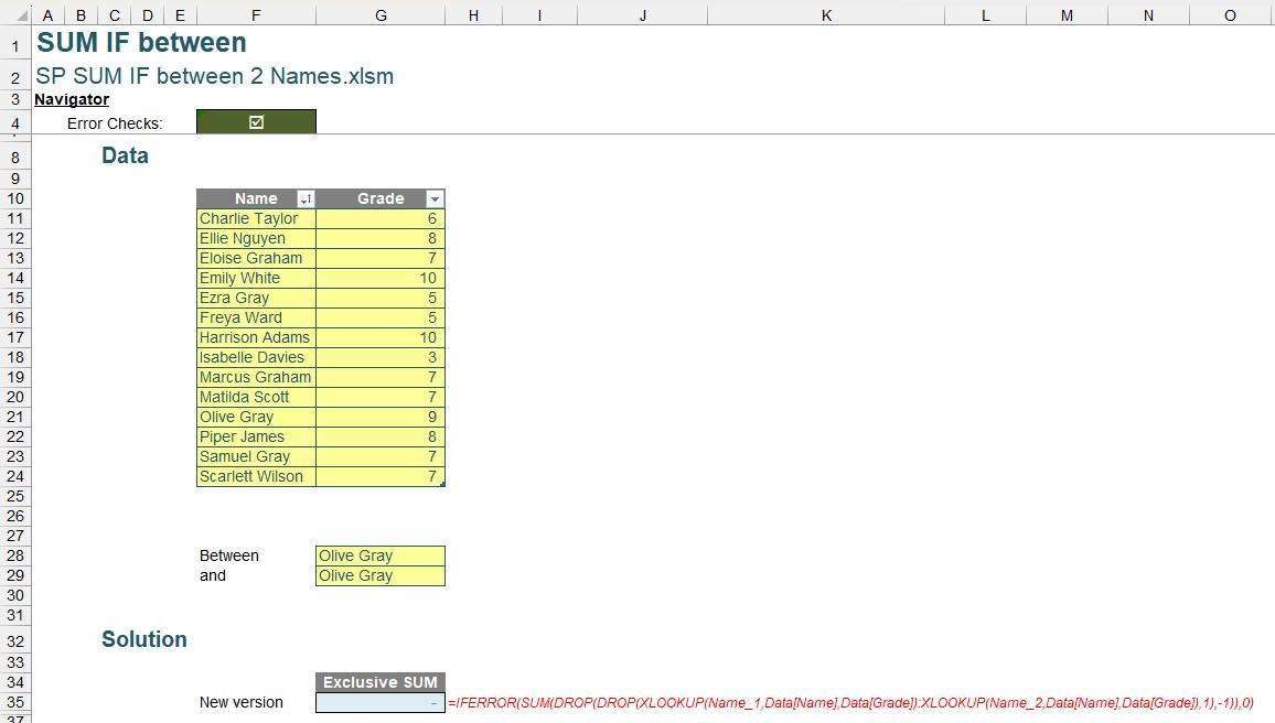
This formula not only performs the desired summation but also ensures that in cases where our formula would return an error, it returns a zero [0] instead.
We have created a resilient, dynamic and accurate formula that sums the data between the specified names whilst avoiding any errors.
Suggested Solution for Legacy Excel Users (Older Versions of Excel)
You can find our Excel file here, which shows our suggested solution. The steps are detailed below.
Using INDEX MATCH and Colon to Create a Data Range
In a manner akin to the approach for modern Excel users, we will use the INDEX MATCH partnership combined with a colon to define the data range. This method uses
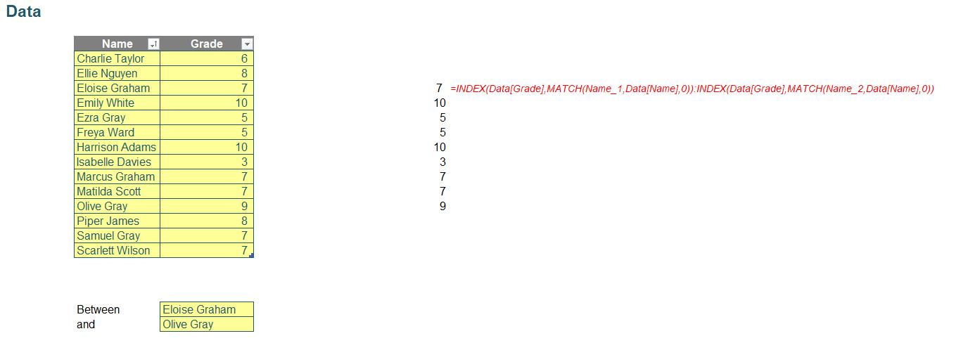
=INDEX(Data[Grade],MATCH(Name_1,Data[Name],0))
to locate the grade for Name_1. Similarly,
=INDEX(Data[Grade],MATCH(Name_2,Data[Name],0))
The above formula is employed to find the grade for Name_2.
Placing a colon between these two [2] formulae creates a range spanning from the grade of Name_1 to Name_2, viz.
=INDEX(Data[Grade],MATCH(Name_1,Data[Name],0)):INDEX(Data[Grade],MATCH(Name_2,Data[Name],0))
Making it Exclusive
To exclusively select the data between Name_1 and Name_2, we introduce the MAX and MIN functions. These functions are employed to determine the endpoints of our data range:
=MAX(MATCH(Name_1,Data[Name],0),MATCH(Name_2,Data[Name],0))
This formula is used to find the last position in the data range.
=MIN(MATCH(Name_1,Data[Name],0),MATCH(Name_2,Data[Name],0))
Similarly, this above formula identifies the first position.
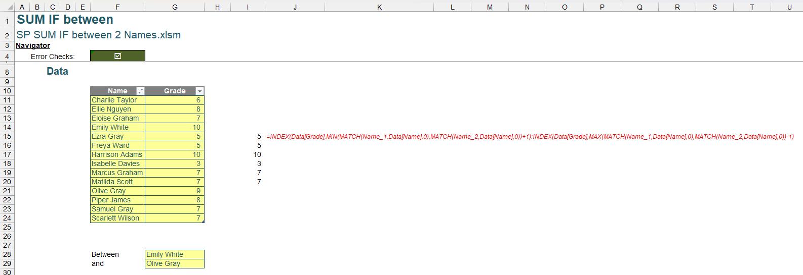
Subsequently, we modify our original INDEX:INDEX formula to replicate the effect of the DROP function used in the modern Excel solution:
=INDEX(Data[Grade],MIN(MATCH(Name_1,Data[Name],0),MATCH(Name_2,Data[Name],0))+1):
INDEX(Data[Grade],MAX(MATCH(Name_1,Data[Name],0),MATCH(Name_2,Data[Name],0))-1)
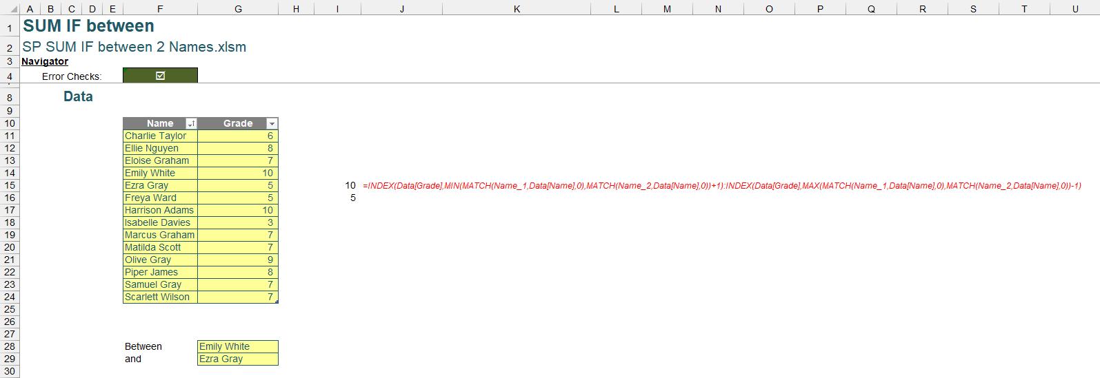
Addressing Specific Selection Scenarios
While effective, our method may not be perfect in all cases. For instance, if Name_1 and Name_2 are adjacent, the same name is selected twice or the input cells are left empty, the formula might produce an incorrect range or result in an error.
To address this, we implement the following formula:
=IFERROR(ABS(MATCH(Name_1,Data[Name],0)-MATCH(Name_2,Data[Name],0)),0)<=1
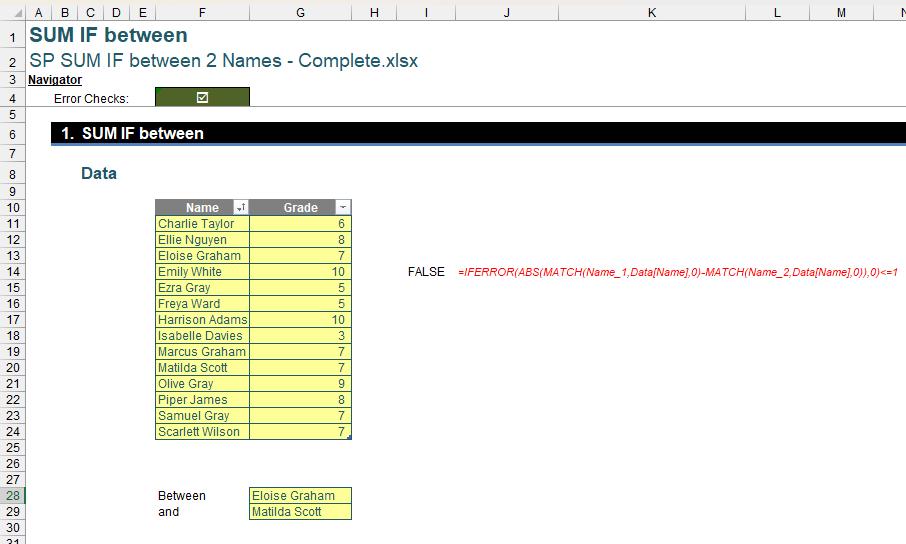
This formula utilises ABS and MATCH functions to detect if Name_1 and Name_2 are adjacent or identical. Additionally, the IFERROR function will intercept any #N/A errors from the MATCH function being unable to match any name and then convert them to zero [0]. The subsequent comparison (<=1) checks if the range is suitable for summation. We encapsulate this logic within a comprehensive IF statement:
=IF(IFERROR(ABS(MATCH(Name_1,Data[Name],0)-MATCH(Name_2,Data[Name],0)),0)<=1, 0, SUM(INDEX(Data[Grade], MIN(MATCH(Name_1,Data[Name],0),MATCH(Name_2,Data[Name],0))+1) : INDEX(Data[Grade], MAX(MATCH(Name_1,Data[Name],0),MATCH(Name_2,Data[Name],0))-1)))
This approach ensures an accurate and exclusive summation between the selected names, catering to the nuances of legacy Excel.
Word to the Wise
We appreciate there are many, many ways this could have been achieved. If you have come up with an alternative, radically different approach, congratulations – that’s half the fun of Excel!
The Final Friday Fix will return on Friday 29 March 2024 with a new Excel Challenge. In the meantime, please look out for the Daily Excel Tip on our home page and watch out for a new blog every business working day.