
Monday Morning Mulling: December 2022 Challenge
26 December 2022
Merry Christmas and Happy New Year! On the final Friday of each month, we set an Excel / Power Pivot / Power Query / Power BI problem for you to puzzle over for the weekend. On the Monday, we publish a solution. If you think there is an alternative answer, feel free to email us. We’ll feel free to ignore you.
The challenge this month was to create a Secret Santa game in Excel. Did you make it?

The Challenge
Merry Christmas and Happy New Year, everyone! It is the time of the year again for many get together and celebrate the holiday season. The gift-exchanging ritual may be an indispensable part for some. So how do we usually exchange a gift? Well, some might say Secret Santa is the way to go. Hence, we took this opportunity to issue a challenge for you to build a Secret Santa game.
For those who are not familiar with the term “Secret Santa”, this game essentially is a game where everyone writes down their name on a piece of paper and each player draws a random name out of a hat and you will be the Secret Santa for that person on the piece of paper.
We challenged you to rebuild the Secret Santa game using
only the Excel formula. You could
download the question data here.
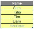
This December’s challenge was to write some formulae to split a list of players into pairs of senders (Secret Santa) and recipients of gifts. The Players table was as follows:
As always, there were some requirements:
- this was a formula challenge; no Power Query / Get & Transform or VBA
- a maximum of one [1] helper column is allowed
- the formula should be dynamic enough to update when a new name was added
- a gift’s sender could not be the same as its receiver
- each person should receive one and only one gift.
Suggested Solutions
You can find our Excel file here, which shows our suggested solutions. Before we discuss the solutions, we would like to note some complicated issues here. Let’s go through them.
Problem 1: Which Random Functions?
To replicate the random draw, we will need to employ the random formula of Excel. The question now is which random formula we should use here? There are three [3] random functions that generate random numbers in Excel:
- RAND: generates a random number between zero [0] and one [1]
- RANDARRAY: produces an array of random numbers based upon specific conditions
- RANDBETWEEN: returns a random integer between two specified numbers.
All these three [3] can help us create a new random series of numbers which later we can use the RANK / RANK.EQ or SORTBY functions to shuffle the original list by the random series of numbers.
Problem 2: Taming Randomness
When undertaking the challenge, you might want to combine more than two [2] random functions within your formula. Then the result is a terrible disaster. For example, if we try to compare two [2] RAND functions here:
=RAND() = RAND()
most of the time the result will be FALSE, although in some rare cases we will get the result TRUE. If we need to use more than two [2] random functions within our formula, we will need to set it up so that all the random number generators within the formula produce the same result.
Problem 3: Our Own Secret Santa
This might be the well-known problem that is when we play Secret Santa, some players might get their own gift. This is not allowed for the purposes of this game! The random number generator you build needs to account for this real-life dilemma where no one is left on their lonesome.
Brainstorming
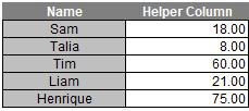
To answer the first problem, we will use the RANDBETWEEN function. The reason we choose the RANDBETWEEN function as our random generator is that we want to avoid using heavy rank sorting using COUNTIF later (you can find out more about the use of RANK and COUNTIF functions to deal with duplicated random numbers here). We will generate a list of distinct random numbers as follows instead:
=RANDBETWEEN(1,100)+ROW()/1500000
where:
- RANDBETWEEN(1,100) helps us generate a random integer number from one [1] to 100
- ROW()/1500000 takes the current row numbers divided by 1.5 million. There are a maximum of 1,048,576 rows in one Excel Spreadsheet, hence this expression ROW()/1500000 will always be smaller than one [1] (yes, we know the choice of number is arbitrary – that’s the point!). Since the first component generates integers from one [1] to 100, keeping the second component less than one [1] will ensure it does not interfere with the first component. This will make sure the higher row number will have a lower rank than the lower row number if the first components ever return the same value.
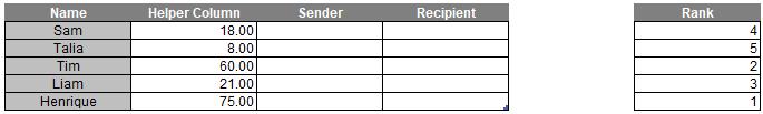
Next, what we need is to rank these random numbers, so we will use the RANK function here (You can use the SORT or SORTBY function here to achieve the same desired result):
=RANK(Solution[@[Helper Column]],Solution[Helper Column])
This formula will give us the following visual:
Backed to Suggested Solutions
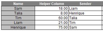
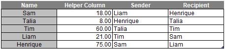
By using the RANK formula, we will rank our random number series in the ‘Helper Column’ from one [1] to the number of players we have here. Then we can use the INDEX function to rearrange the name in the Name column:
=INDEX([Name],RANK([@[Helper Column]],[Helper Column]))
Hence, in the Sender column we will enter the above formula to get the following result:
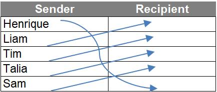
What we essentially did here is we took the people from the Players column and place them randomly in the Sender column. Next, we will offset the name in the Sender column one [1] row up (you can offset one [1] row down if you want here). Hence, the first person on the Sender list will be the last person on the Recipient and everyone else will move one [1] row up:
To perform that offset we will apply the MOD function (assuming the names start on row 23 – please see attached Excel file):
=MOD(ROWS(E$23:E23),ROWS([Name])) + 1
where:
- ROWS(E$23:E23) formula here will generate the number of the row(s) we currently evaluate. Therefore, for the current formula, it will return the value of one [1]. If we drag this formula down in a table, it will generate a series of numbers from one [1] to five [5] which is the total number of players we have
- ROWS([Name]) is the total number of players we have
- The MOD function will take the remainder after the number is divided by the divisor which gives us the following:
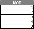
After adding one [1] to the MOD function, we will have the following results:
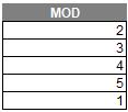
This is the offset that we wanted! Now, we will wrap this MOD function around by the INDEX function as below.
=INDEX([Sender], MOD(ROWS(E$23:E23),ROWS([Name])) + 1)
As you can see here the Recipient is the result of offsetting the Sender list by one [1] row. Thus, we have solved the Secret Santa dilemma! For those who wish to challenge themselves, they might go further by just using one [1] single formula to solve this problem. Well, we also have a suggestive solution for that as well.
Alternative Solution
This solution uses the LET function, which is a function that is only available in Excel 365, Excel Online or Excel 2021. The LET function allows us to name the results of the calculations and store the intermediate calculations, values or defined names inside a formula. Hence, we will use the LET function as follow for our single formula:
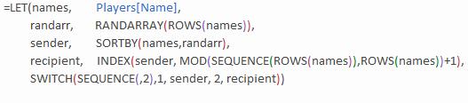
=LET(names, Players[Name],
randarr, RANDARRAY(ROWS(names)),
sender, SORTBY(names, randarr),
recipient, INDEX(sender, MOD(SEQUENCE(ROWS(names)),ROWS(names))+1),
SWITCH(SEQUENCE(, 2), 1, sender, 2, recipient))
where:
- names: this refers to the Players list we have
- randarr: this is the random number generator we use
- sender: this returns the names that have been sorted by the randarr. This replicates what we did for the Sender column in the standard solution where we sort the Name column by the ‘Helper Column’ using the RANK function
- recipient: this moves the sender by one [1] row up, which replicates what we did for the Recipient column in the standard solution
- The last component, SWITCH function will send the result into a two-column array where sender is in the first column and the recipient is in the second column.
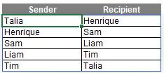
This solution will give us the following array:
Word to the Wise
You may notice that our solutions are not perfect. What our solutions generally do is randomly place people in a circle and they will give the present to the person on their left (or their right), which works fine since it solves the Secret Santa problem of receiving your own gift. Nevertheless, these solutions omit some of the great gift-giving cases we might have for Secret Santa.
What our solutions offer is like this diagram:

In real life, sometimes Secret Santa can have this dynamic of gift-giving:

As we can see here A, B, C and D create a close circle of gift giving and E and F create a similar close circle of gift giving. This can totally happen during Secret Santa, and everyone receives a present. Perhaps this could be an idea for another Final Friday Fix.
The Final Friday Fix will return on Friday 27 January 2023 with a new Excel Challenge. In the meantime, please look out for the Daily Excel Tip on our home page and watch out for a new blog every business working day.