Monday Morning Mulling: August 2022 Challenge

On the final Friday of each month, we set an Excel / Power Pivot / Power Query / Power BI problem for you to puzzle over for the weekend.  On the Monday, we publish a solution.  If you think there is an alternative answer, feel free to email us.  We’ll feel free to ignore you.

The challenge this month was to standardise column names and append the source files together.  Did you succeed?

The Challenge

This month, we had a Power Query challenge.  There were three [3] transactions files of different entities exported from an accounting system.  Our goal was to combine them all together into a master table.

However, we had some “issues”:

• they do not have the same number of columns; and
• some column names are a little bit different depending on which country the entities are located in. 

We provided the challenge files here.

Therefore, this month’s challenge was to extract the files from a given folder, standardise the column names and append them together.  The result should have looked like the table generated at the bottom of the picture below:

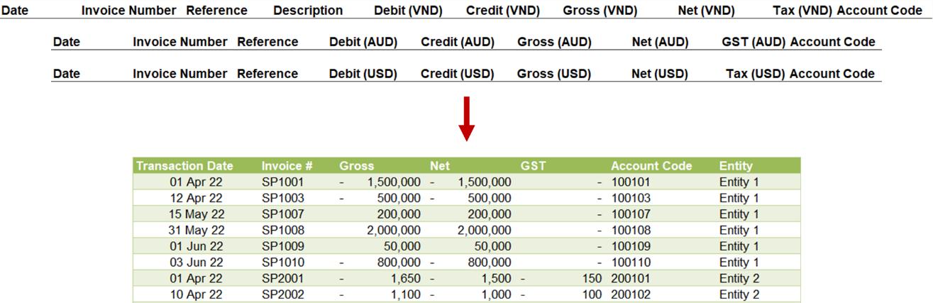
As always, there were some conditions:

• it should be possible for more source files to be added to the folder in the future
• each file can have a different number of columns
• the entity name should be extracted to an addition column
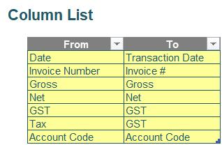
• only some columns are needed, and are listed in the ColumnList table (below)
• GST and Tax are presumed to be the same column
• some columns need to be dynamically renamed such as Date and ‘Invoice Number’.  New names are specified in the column To of the table (below).

Suggested Solution

You can find our Excel file here which demonstrates our suggested solution.

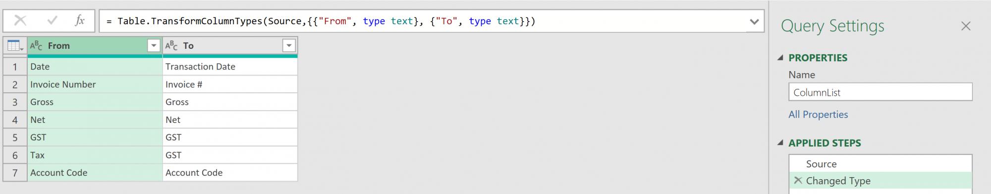
We start by extracting table ColumnList of the challenge file into Power Query:

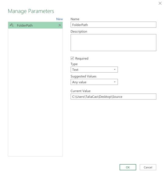
Before getting data from a folder, we create a new parameter called FolderPath.  The ‘Current Value’ of the parameter is the folder path in your PC after you have downloaded and unzipped the Source folder.

Now, we can start getting files from the Source folder as usual.  The hard-coded path on the Formula bar needs to be replaced with the parameter we have just created.

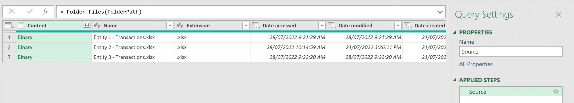
Next, we click the ‘Combine Files’ button next to Content column to start combining files.

We select Transactions sheet on the pop-up dialog and click OK.  Power Query will automatically generate some new queries.  Due to the complexity of the source files, we need to cleanse data from the Transform Sample File query before continuing with the main Source query.  We start by removing the ‘Promoted Headers’ step that has been automatically generated, as we will need to remove rows before this step. 

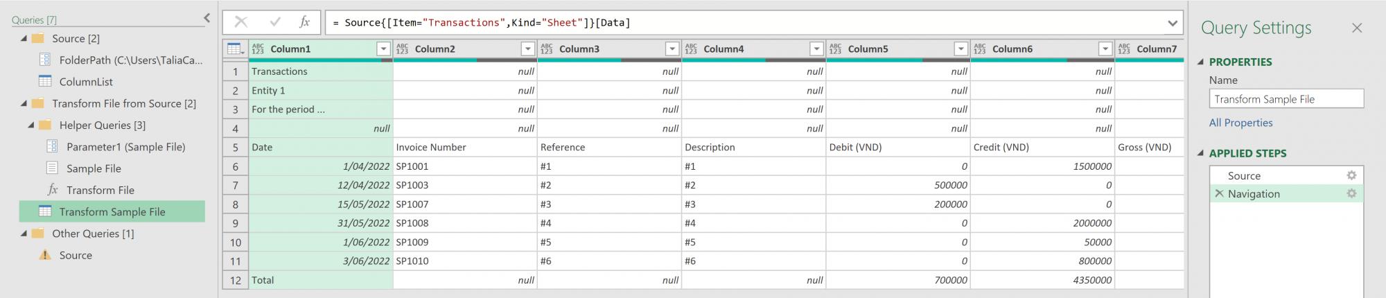
One requirement is to extract the entity name from the header part, but we will just insert a blank step which we call ‘Base’ by clicking the fx symbol next to the Formula bar and come back to this shortly.

We clean this sample file by removing the top four [4] rows and promoting headers.  We remove the autogenerated ‘Changed Type’ step as we do not need it now.

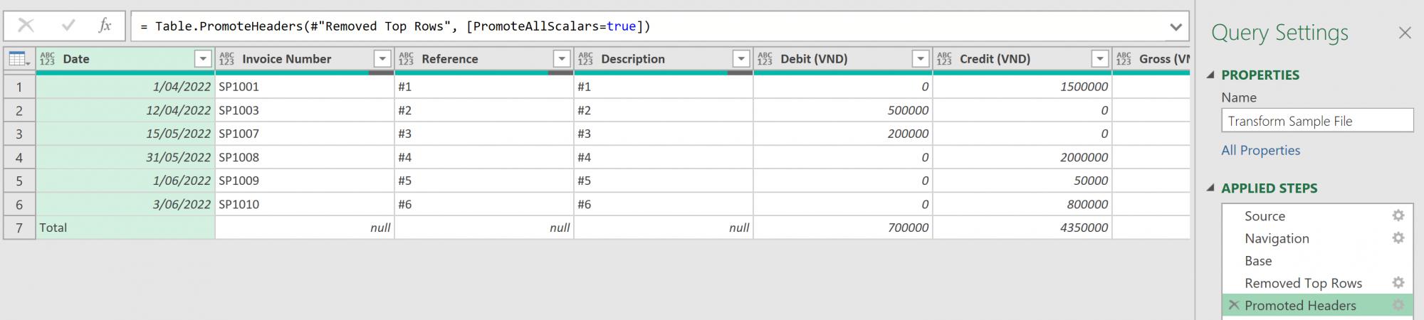
We remove the row containing the totals by filtering out null from the ‘Account Code’ column.

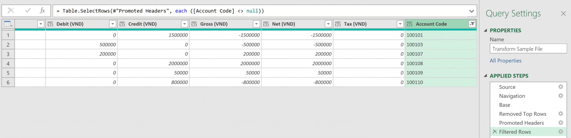
Now, we can standardise column names.

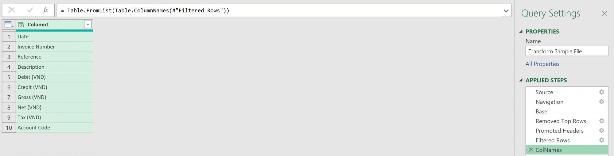
To begin, we add a new blank step with the following M code.  The function Table.ColumnNames gets a list of column names from the ‘Filtered Rows’ step and Table.FromList then converts that list into a table.  We rename this step as ‘ColNames’.

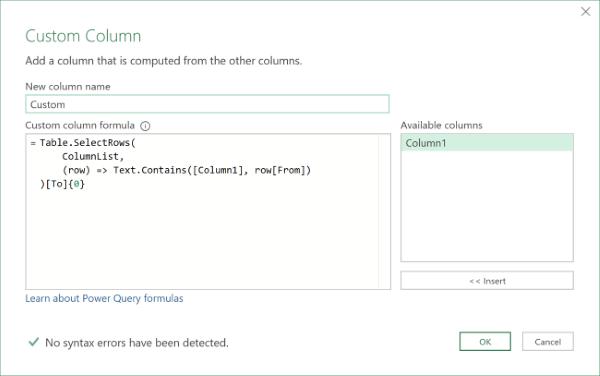
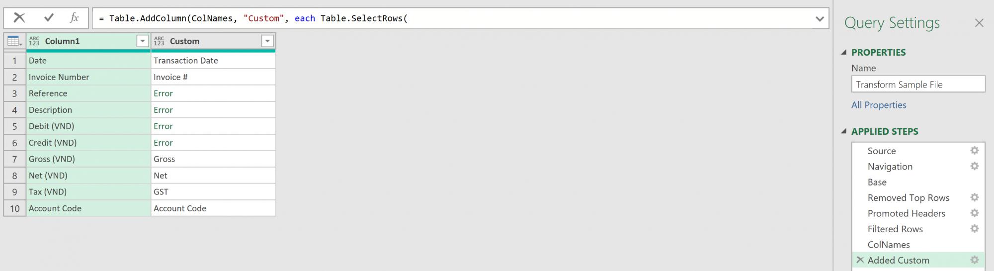
Then, we add a custom column as follows.  Table.SelectRows helps us filter a table by a condition.  The first argument is table ColumnList while the second one contains a function denoted by “() =>” syntax.  This function means that for each row in table ColumnList, Text.Contains checks whether Column1 of the current step contains the value in column From in table ColumnList.  It results in a TRUE / FALSE value which is a condition for the filter.

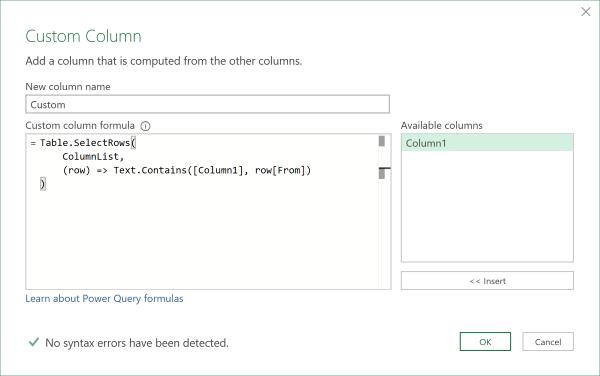
This Custom column generates tables with rows meeting the condition.

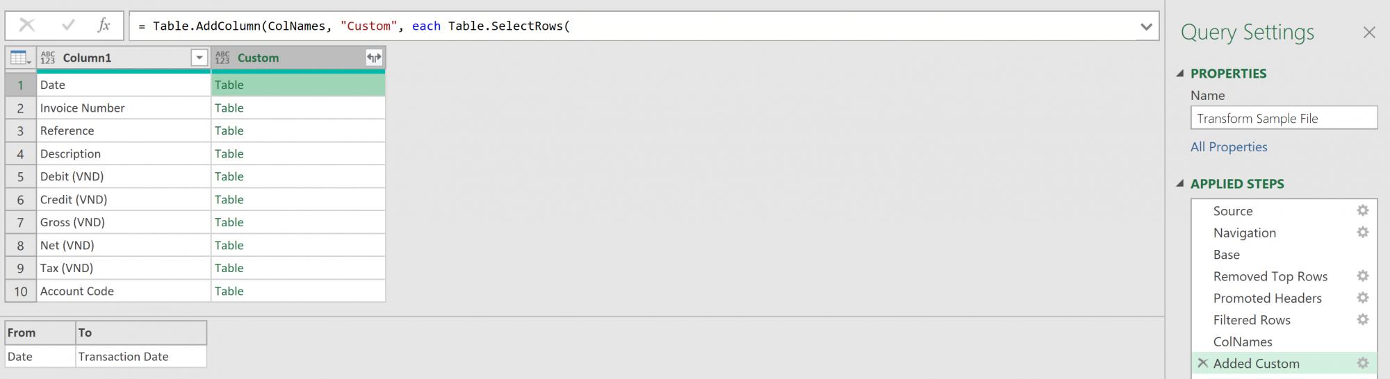
Within these tables, we would like to get the first value of column To by adding “[To]{0}” to the end of the M code.

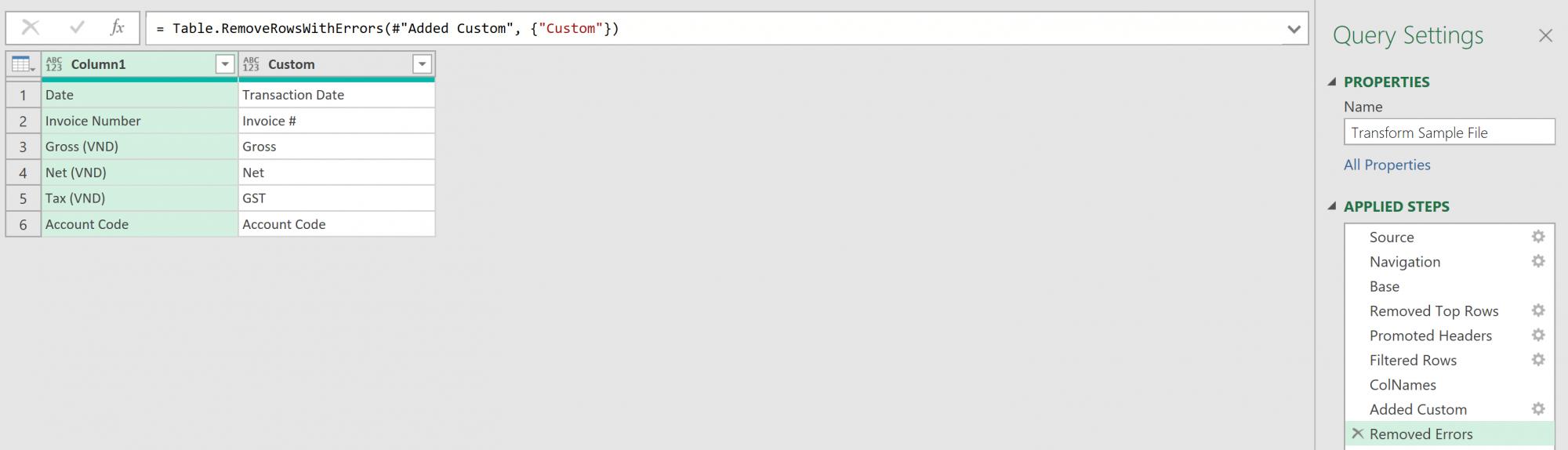
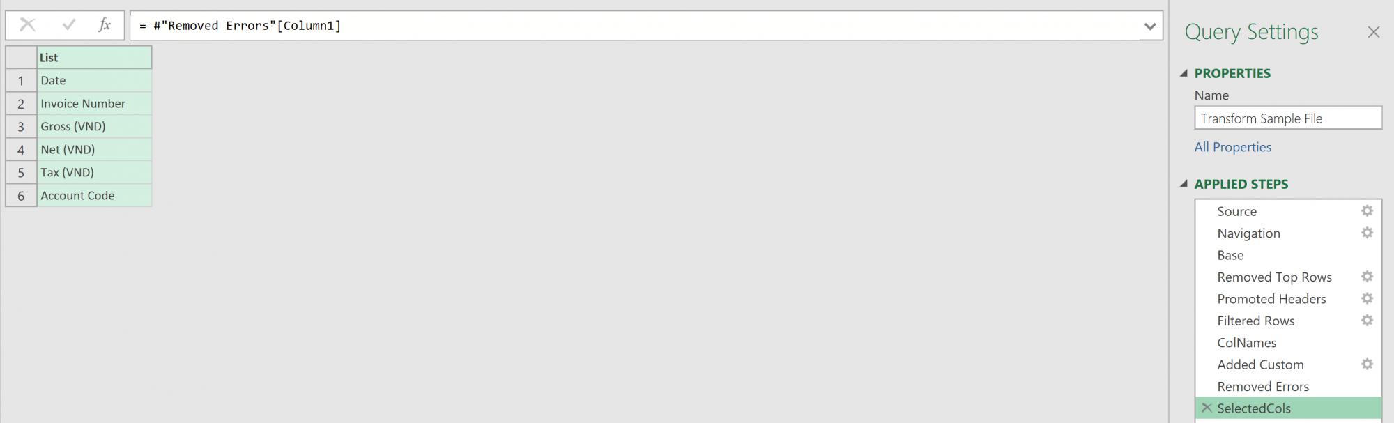
There are some errors for those columns which have no matches from ColumnList.  We do not need these columns, so we apply ‘Remove Errors’ to the Custom column, which means we will be left with a list of columns we want to keep without hardcoding any column names. 

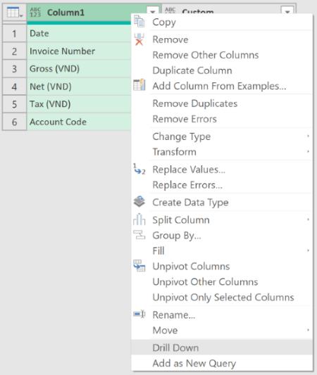
Next, we need to convert Column1 to a list by right-clicking the column header and selecting ‘Drill Down’.  We name the new step as ‘SelectedCols’.

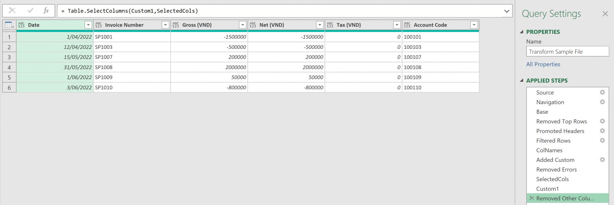
Then, we add a new blank step and refer it back to the ‘Filtered Rows’ step.  We select a few columns to keep and apply ‘Remove Other Columns’ to have Power Query produce the M code below for us.

The hardcoded column list is replaced by SelectedCols as below.

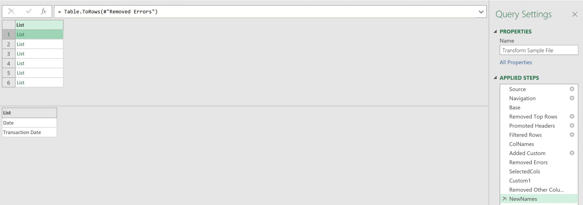
After that, we need to rename the columns.  We create a blank step referring to ‘Removed Errors’ step and edit the step to use a Table.ToRows function to convert the table into a list of lists.  

Each child list contains an old name and its new name.  We rename this step ‘NewNames’.

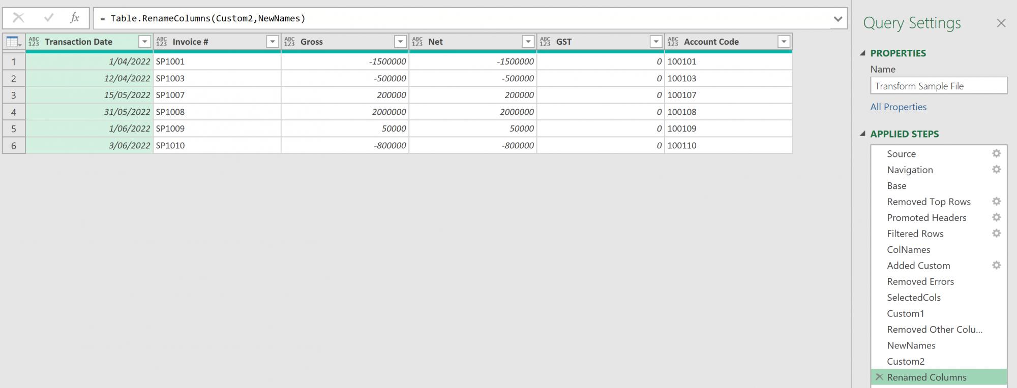
We then create a blank step referring to ‘Removed Other Columns’ step and rename a few columns to get autogenerated M code.  The hardcoded part is replaced by NewNames as follows.

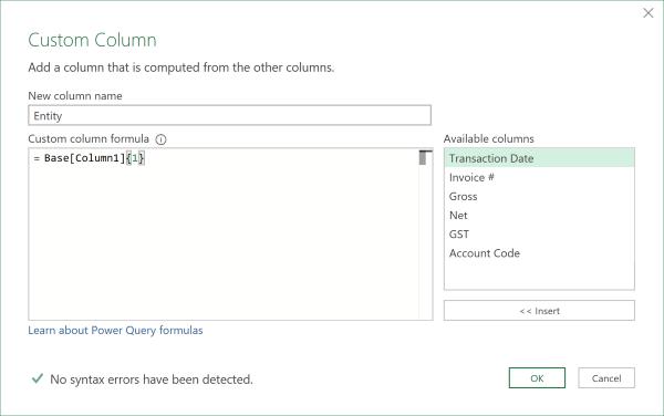
Finally, we add a custom column Entity.  The code below refers to Column1 and the second row of ‘Base’ step where entity name is located.

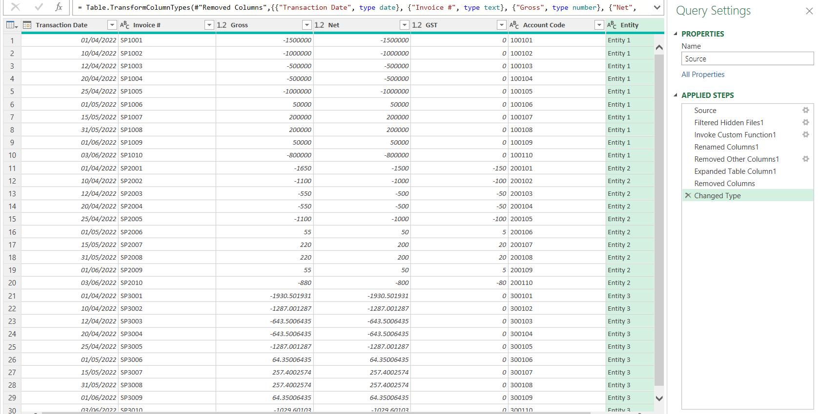
Congratulations!  At this time, the ‘Transform Sample File’ query is complete.  Let’s now return to the main Source query.

There is an error in the automatically generated  ‘Changed Type’ step as the Transactions column no longer exists.  We can safely delete the ‘Changed Type’ step.  Then, right-click and remove the Source.Name column.  Finally, we should change the column types from ‘Any’ to the appropriate type for each column.

Now, it is ready to ‘Close & Load’.

The Final Friday Fix will return on Friday 30 September 2022 with a new Excel Challenge.  In the meantime, please look out for the Daily Excel Tip on our home page and watch out for a new blog every business working day.