
Monday Morning Mulling: September 2020 Challenge
28 September 2020
On the final Friday of each month, we set an Excel / Power Pivot / Power Query / Power BI problem for you to puzzle over for the weekend. On the Monday, we publish a solution. If you think there is an alternative answer, feel free to email us. We’ll feel free to ignore you.
This month, we look at a common “clean up” problem in Excel – how to separate text and numbers.
The Challenge
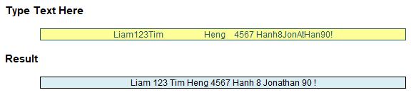
Often, we receive data that isn’t in the best of shape. It may have text and numbers intermingled and you wish to separate (i.e. space) them out. For example, you might want “Pelham123” to be “Pelham 123”, or require “121Training” to be “121 Training”.
Where there is just the one change of data type in the text string, it’s possible to create a reasonably straightforward formula, but things get harder with multiple occurrences. And that’s what this month’s challenge is – fix the issue in general.
Using your favourite search engine will typically yield third party add-ins, VBA (e.g. User Defined Functions) and Power Query solutions – all NOT allowed here!
This month’s challenge is to construct an Excel formula that will split out multiple occurrences of numbers and text, e.g.
To aid understanding of our suggested solution, please feel free to refer to the associated Excel file.
Suggested Solution
This problem has been a regular challenge for Excel users since the dawn of time. Well, 1985 anyway. >Dynamic arrays have made the task easier because you can now undertake repetitive checks. Dynamic arrays have made the task easier because you can now undertake repetitive checks. Dynamic arrays have made the task easier because you can now undertake repetitive checks…
OK, joke’s over.
Using the associated Excel file, you can see our suggested solution is extremely simple:
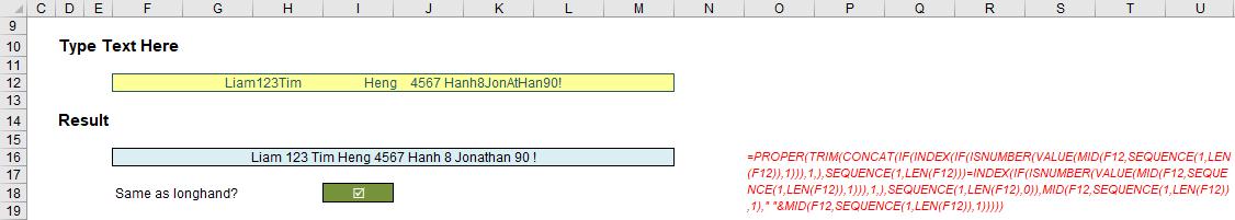
=PROPER(TRIM(CONCAT(IF(INDEX(IF(ISNUMBER(VALUE(MID(F12,SEQUENCE(1,LEN(F12)),1))),1,),SEQUENCE(1,LEN(F12)))=INDEX(IF(ISNUMBER(VALUE(MID(F12,SEQUENCE(1,LEN(F12)),1))),1,),SEQUENCE(1,LEN(F12),0)),MID(F12,SEQUENCE(1,LEN(F12)),1)," "&MID(F12,SEQUENCE(1,LEN(F12)),1)))))
Any questions?
Perhaps we need to step through this monster.
In the attached Excel file, the second section steps through the mechanics of this calculation. The first formula is (hopefully) straightforward!

If you need help with this calculation, then the rest of this explanation is not looking good. This simply links the original input into cell P28, so all the formulae are close together. That’s not so exciting.
The next formula is a tad more interesting:

Even in this stepped out approach, I have managed to include three functions in one formula!
- LEN(P28) is a text function that counts the number of characters (its “volume”) in the text string in cell P28. In the example (above), there are 58 characters, so LEN(P28) equals 58
- The SEQUENCE(rows, [columns], [start], [step]) function has one required (rows) and three optional arguments. This is one of the new >dynamic array functions and fills rows number of rows, columns number of columns (1 if not specified), starting at start (1 if not specified) in increments of step (1 if not specified). Hence, =SEQUENCE(4,3,2,1) would be
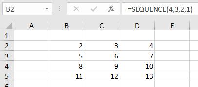
It would consist of 12 cells (4 rows by 3 columns), starting with the number 2 and increasing in increments of 1 (as pictured).
Therefore, = SEQUENCE(1,LEN(P28)) would be the numbers 1 to 58, all in one row, across 58 columns
- Finally, =MID(P28,SEQUENCE(1,LEN(P28)),1) uses the MID(text, start_number, length) function. Here, it takes a sub-text string from the text reference, starting at position start_number of length length. So, =MID(“abcdefg”,2,3) would be “bcd” being three characters starting from the second position.
Therefore, =MID(P28,SEQUENCE(1,LEN(P28)),1) simply splits the text string out into 58 cells across a row, each cell consisting of just one of the 58 characters in the text string. It should be noted that MID converts every element to a text string, i.e. all characters are text – even numbers.
You can read more about the text functions LEN and MID here.
Let’s look at the next two formulae together:
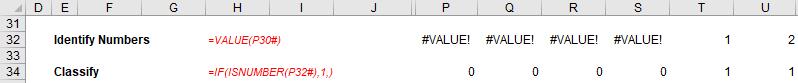
=VALUE(P30#)
=IF(ISNUMBER(P32#),1,)
I want to identify which characters are numbers in the range starting in cell P30 (P30# simply means the spilled dynamic array, so all 58 cells – but this will change if the text length changes). ISNUMBER will do this – but not straight away. Remember, MID has converted everything to text, so first I need to convert numbers back to numbers.
Interestingly, the N function won’t work here (it will “coerce” the range back to one cell), but VALUE will. Values of text characters are #VALUE! by definition.
Then, with this new range in P32#, we can see what is a number and what isn’t. The formula
=IF(ISNUMBER(P32#),1,)
Simply provides a 1 for every numerical value and zero (0) for everything else (including #VALUE! errors).
The next three steps may be considered together:
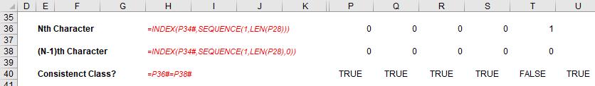
=INDEX(P34#,SEQUENCE(1,LEN(P28)))
=INDEX(P34#,SEQUENCE(1,LEN(P28),0))
=P36#=P38#
The expression =SEQUENCE(1,LEN(P28)) has already been explained: this generates the numbers 1 to 58 in 58 cells across the row. Since P34# contains 58 cells across one row,
=INDEX(P34#,SEQUENCE(1,LEN(P28)))
is a seemingly rather longwinded way of replicating P34# - the first cell provides the first value in the vector P34#, the second cell provides the second value in the vector P34# and so on. It seems convoluted. It’s subtle though: this formula is giving us a way of referencing a particular position in the range P34#. That’s important when we consider the second formula:
=INDEX(P34#,SEQUENCE(1,LEN(P28),0))
Almost the same formula, the start of zero (0) is specified in the SEQUENCE function. When it is not specified (as in the first formula considered in this section), it is assumed to start at one (1). This has the effect of producing the same result as the first formula, albeit displaced one cell to the right, e.g. the first cell provides the “noughth” value in the vector P34#, the second cell provides the first value in the vector P34#, and so on. In other words, it displays the previous cell result.
The formula
=P36#=P38#
simply checks that the current cell and the previous cell in the range are both text or both numerical values (TRUE). If they differ, the result is FALSE. This is what we want to find. Wherever we have a FALSE value, we need to add a space to separate text and numbers (or vice versa). This is precisely what the next formula does:

=IF(INDEX(P34#,SEQUENCE(1,LEN(P28)))=INDEX(P34#,SEQUENCE(1,LEN(P28),0)),P30#," "&P30#)
This formula takes the logic of the above. The formula =P36#=P38# cannot be referred to per se (it has been provided for illustration) as this is not how dynamic arrays work. However, this formula checks for inconsistent data types between the cell and the prior and adds a preceding space if the two data types differ (i.e. the equality is FALSE). For example, the value in cell T42 is not 1, but “ 1” (i.e. it has a preceding space to delineate between text and number).
The final three formulae simply tidy things up:
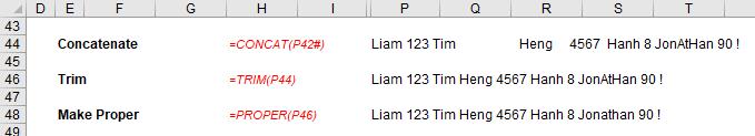
=CONCAT(P42#)
=TRIM(P44)
=PROPER(P46)
The formula in cell P44 simply combines all the cell values back into one cell using the CONCAT (concatenate) function; the formula on cell P46 removes excess spaces using TRIM; the final formula in cell P48 just puts all text into “Proper” case, i.e. each word starts with a capital letter, with all other letters using lower case.
That’s it.
To get the monster formula, you just build each formula into its dependent calculation so the last formula could be expressed as
=PROPER(TRIM(P44))
and the formula before that could be written as
=PROPER(TRIM(CONCAT(P42#)))
If you carry on this approach, this will eventually result in our monster formula, viz.
=PROPER(TRIM(CONCAT(IF(INDEX(IF(ISNUMBER(VALUE(MID(F12,SEQUENCE(1,LEN(F12)),1))),1,),SEQUENCE(1,LEN(F12)))=INDEX(IF(ISNUMBER(VALUE(MID(F12,SEQUENCE(1,LEN(F12)),1))),1,),SEQUENCE(1,LEN(F12),0)),MID(F12,SEQUENCE(1,LEN(F12)),1)," "&MID(F12,SEQUENCE(1,LEN(F12)),1)))))
Word to the Wise
Dynamic arrays are only supported in Microsoft 365 presently. If you have an earlier version of Excel, the attached Excel file will neither display correctly nor calculate appropriately. In this case, you will have to revert to VBA (e.g. as User Defined Function), a third party add-in or Power Query.
For the time being!
Until next month!
The Final Friday Fix will return on Friday 30 October with a new Excel Challenge. In the meantime, please look out for the Daily Excel Tip on our home page and watch out for a new blog every business workday.