
Monday Morning Mulling: August 2021 Challenge
30 August 2021
On the final Friday of each month, we set an Excel / Power Pivot / Power Query / Power BI problem for you to puzzle over for the weekend. On the Monday, we publish a solution. If you think there is an alternative answer, feel free to email us. We’ll feel free to ignore you.
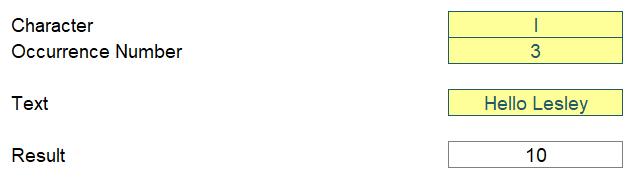
This month, we just wanted you to identify the nth occurrence of a character in a text string. Easy, yes?
The Challenge
Sometimes when modelling you need to identify the location of the nth occurrence of a character in a text string, perhaps to truncate the text or to manipulate it in some other fashion.
This month’s challenge was to write a formula in one cell that would identify the nth occurrence of a character in a text string. There were some constraints:
- the formula needed to be in just one cell (no “helper” cells)
- this was a formula challenge – so no Power Query / Get & Transform or Text to Columns!
- the formula must work in all current versions of Excel (so no VBA, dynamic arrays, LAMBDA, LET or user defined functions)
- the model may be large or unstable, so no volatile functions were allowed
- the formula must be case sensitive. For example, in the illustration above the third occurrence of “l” in “Hello Lesley” is in position 10, i.e. “Hello Lesley” – the capital “L” is ignored.
There were bonus points too: as an additional challenge, a second formula was sought to locate the last occurrence in the same text string too, subject to the same above restrictions.
Our attached Excel file demonstrates our suggested solution(s).
Suggested Solution
There are two common functions in Excel that allow you to rummage through a given text string:
- SEARCH(find_text, within_text, [start_number]) is a search function which is not case sensitive, but does allow for wildcard characters. It seeks out the first instance of a character or characters (typed in inverted commas) in the within_text text string. The start_number argument is optional (hence the square brackets in the syntax), so that the first few characters in a text string may be ignored. If the find_text cannot be located within within_text, the error #VALUE! is returned
- FIND(find_text, within_text, [start_number]) is another search function which is case sensitive, but does not allow wildcard characters. It seeks out the first instance of a character or characters (typed in inverted commas) in the within_text text string. The start_number argument is optional (hence the square brackets in the syntax), so that the first few characters in a text string may be ignored. If the find_text cannot be located within within_text the error #VALUE! is returned.
Here, we need to create a formula that is case sensitive, which therefore forces us to use FIND rather than SEARCH (we do not need to consider wild cards here). The problem is, like its SEARCH counterpart, FIND seeks out the first occurrence of find_text – so we will need to be crafty.
If we cannot find the nth occurrence of a character (find_text) within a text string (within_text), then we need to locate the nth occurrence of the character and replace it with an alternative character that we KNOW will occur once and only once in the text string. Then, we may simply FIND this character.
But what character should we use as the replacement? We need it to be one that cannot be easily typed into a cell. A cursory glance of the internet will suggest @ or CHAR(160), the non-breaking space (often used in HTML code). I would suggest neither:
- @ is now a special character associated with dynamic arrays / legacy formulae in some versions of Excel and may be problematic
- CHAR(160) causes problems with some text functions in Excel already, such as TRIM which cannot remove it, and therefore is best avoided.
I am going to suggest CHAR(1), which is the unprintable “Start of Heading” character in the ASCII system. I don’t think anyone will be typing this into a text string!
So how do we replace the nth occurrence of a given character with CHAR(1)? Two common functions come to mind:
- REPLACE(old_text, start_number, number_of_characters, new_text) is a function that allows you to swap one or several characters in a text string with another character or a set of characters. In the old_text, it seeks out the characters to be swapped by starting at the start_number of the text string and replacing the number_of_characters with the new text.
For example,
=REPLACE(“Get the answer next time”,5,10,”it right”)
becomes “Get it right next time”
- SUBSTITUTE(text, old_text, new_text, [instance_number]) is similar to REPLACE, as it replaces one or more instances of a given character or text string (old_text) in a text string with a specified character or string (new_text). The optional instance_number cites the occurrence of old_text you wish to replace. If this is omitted, all occurrences will be replaced, viz.
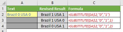
Only SUBSTITUTE allows us to specify the instance_number – but that’s enough: we now have a plan of attack.
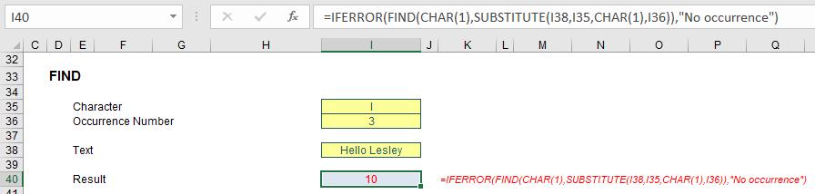
In the example illustrated (above), I have used the formula
=IFERROR(FIND(CHAR(1),SUBSTITUTE(I38,I35,CHAR(1),I36)),"No occurrence")
To explain how this works:
- SUBSTITUTE(I38,I35,CHAR(1),I36) substitutes the third (I36) occurrence of “l” (I35) with CHAR(1) in the text “Hello Lesley” in cell I38. This now guarantees only one occurrence of the character which now occupies the position that needs to be identified
- FIND(CHAR(1),SUBSTITUTE(I38,I35,CHAR(1),I36)) then returns the position of this unique character CHAR(1)
- IFERROR(FIND(CHAR(1),SUBSTITUTE(I38,I35,CHAR(1),I36)),"No occurrence") simply provides an error trap should there be no occurrence of the desired character (cell I35).
Taking this challenge one step further, to find the last occurrence is slightly trickier as we don’t know how many occurrences there are. You could construct a calculation to reverse the text string, but the formula I have used is as follows:
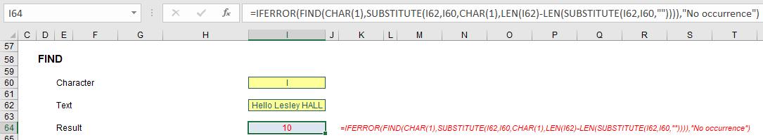
Perhaps not the largest graphic ever committed to an article, but the formula is given by
=IFERROR(FIND(CHAR(1),SUBSTITUTE(I62,I60,CHAR(1),LEN(I62)-LEN(SUBSTITUTE(I62,I60,"")))),"No occurrence")
This works similarly to the earlier calculation:
- SUBSTITUTE(I62,I60,""): this element replaces the selected character with an empty string
- LEN(I62)-LEN(SUBSTITUTE(I62,I60,"")): this calculates how many times the selected character occurs in the string. This is because this formula subtracts the length of the string without any occurrences of the character (since all instances are replaced with an empty string) from the length of the original text string with all the original instances of the character intact
- SUBSTITUTE(I62,I60,CHAR(1),LEN(I62)-LEN(SUBSTITUTE(I62,I60,""))): this is where we first came in! We now know how many occurrences there are of our chosen character, and this calculation substitutes the final occurrence of “l” (I60) with CHAR(1) in the text “Hello Lesley HALL” in cell I62. This now guarantees only one occurrence of the character which now occupies the position that needs to be identified
- FIND(CHAR(1),SUBSTITUTE(I62,I60,CHAR(1),LEN(I62)-LEN(SUBSTITUTE(I62,I60,"")))): then returns the position of this unique character CHAR(1)
- IFERROR(FIND(CHAR(1),SUBSTITUTE(I62,I60,CHAR(1),LEN(I62)-LEN(SUBSTITUTE(I62,I60,"")))),"No occurrence"): this simply provides an error trap should there be no occurrence of the desired character (cell I60).
It may seem horrible, but broken down, it’s not so bad.
Word to the Wise
In case you are wondering why this challenge may be at all relevant in the real world, these sort of issue occur all the time. For example, you may have serial numbers such as
ISBN 978-3-16-148410-0-SERIAL-78-8
ISBN 978-1-940313-1-0-2-RADIUS-15-19
ISBN 978-0-7334-2609-PUBL-2-4
and wish to extract the text strings “SERIAL”, “RADIUS” and “PUBL”. This would be possible using extrapolations of the ideas discussed above.
Until next month!
The Final Friday Fix will return on Friday 24 September 2021 with a new Excel Challenge. In the meantime, please look out for the Daily Excel Tip on our home page and watch out for a new blog every business workday.