
Monday Morning Mulling: April 2022 Challenge
2 May 2022
On the final Friday of each month, we set an Excel / Power Pivot / Power Query / Power BI problem for you to puzzle over for the weekend. On the Monday, we publish a solution. If you think there is an alternative answer, feel free to email us. We’ll feel free to ignore you.
The challenge this month was to transform the layout of data from vertical form to horizontal. Easy, yes?
The Challenge
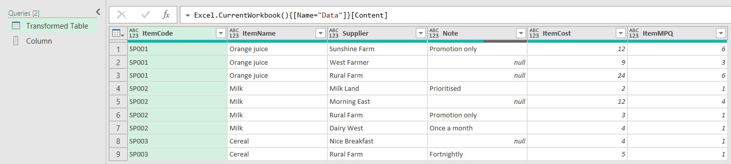
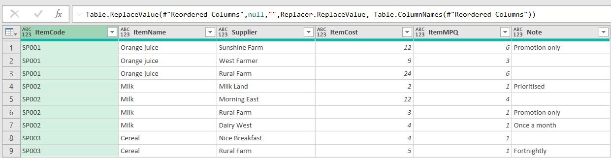
We have a table called ‘Data’ that contains details of some new items and their suppliers in a clean horizontal structure, as below. We need to import this data into an inventory management system.
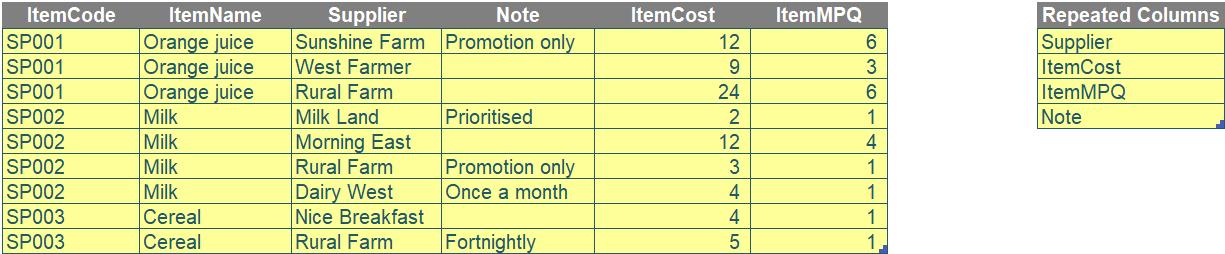
However, the system requires a template that only allows one row per item. Therefore, the data needs to be laid out as follows.

In this challenge, the objective was to use Power Query to transform structure of the data from vertical format to horizontal as shown in the pictures above.
You can download the question file here.
As always, there were some requirements:
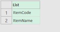
- repeated columns were listed in the second table of Question Data. They had to be in that specific order (i.e. ‘Note’ is the last column of every repeated group)
- all column headers needed to be dynamic. If they were changed, the queries still needed to work
- the number of suppliers for each item may be varied.
Suggested Solution
You can find our Excel file here which demonstrates a suggested solution.
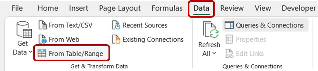
Firstly, we bring two question tables into Power Query, one by one, by selecting each table and then navigating to the Data tab, and click ‘From Table/Range’ under the ‘Get & Transform Data’ grouping, viz.
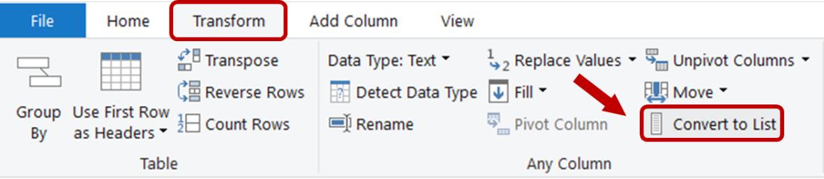
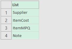
Secondly, we need to convert the ‘Column’ query into a list by going to Transform tab and then selecting ‘Convert to List’.
Thirdly, we come to the Data table. We rename this query ‘Transformed Table’.
We need Power Query to identify a list of grouped columns (i.e.ItemCode and ItemName). To do this, we add a new step by clicking ‘fx’ next to the formula bar. Then, the List.RemoveItems and Table.ColumnNames functions are used to remove all repeated columns listed in the Column list (which we created earlier) from the Source step. We add the formula below to the Formula bar and name this step as GroupCols.
=List.RemoveItems(Table.ColumnNames(Source),Column)
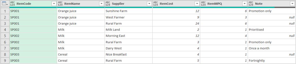
Then, we re-order the columns with the following formula. List.Combine helps combine grouped columns above with the Column list, which has a correct column order for repeated columns.
=Table.ReorderColumns(Source,List.Combine({GroupCols, Column})
As you can see from the picture below, Note is now the last column.
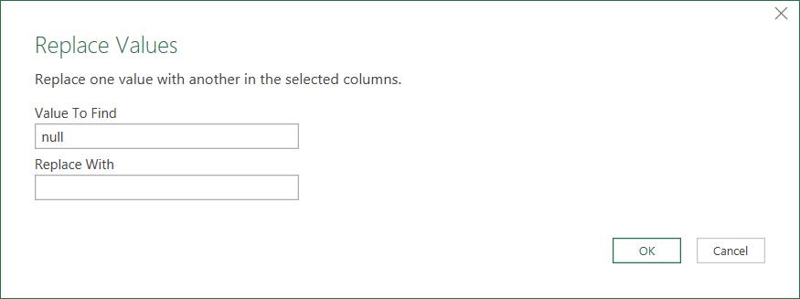
We will next remove all the null values in the table by replacing values null with “”. This ensures that all values are kept after unpivoting later.
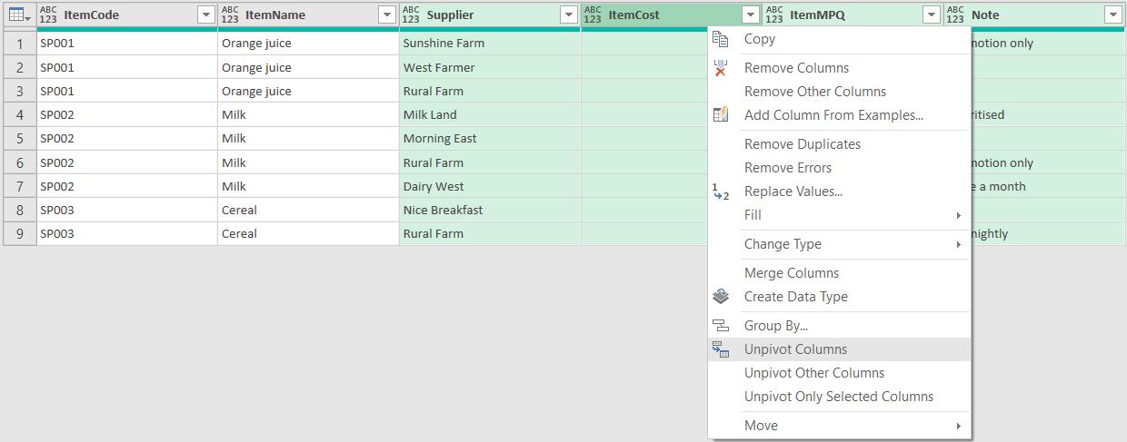
After that, we need to unpivot the columns, specifically the four repeated columns in our ‘Column’ list. We simply select the four columns, right click and select ‘Unpivot Columns’.
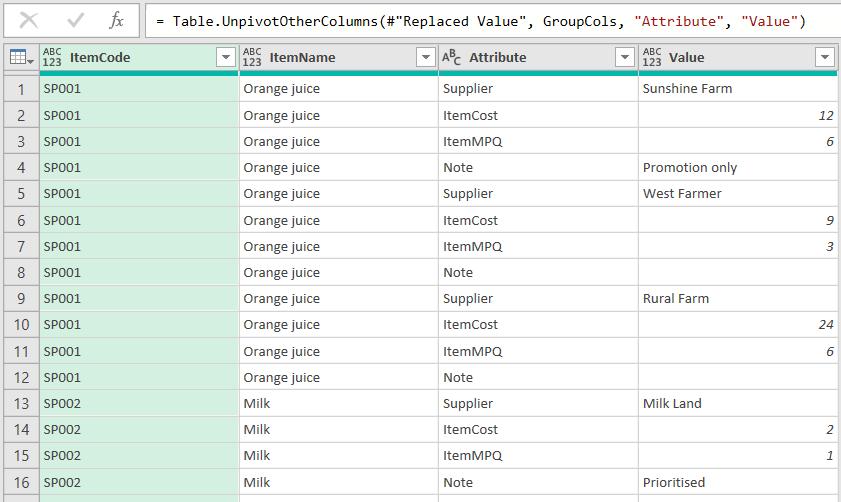
To keep the query dynamic, we need to replace the grouped columns with our variable ‘GroupCols’ from:
= Table.UnpivotOtherColumns(#"Replaced Value", {"ItemCode", "ItemName"}, "Attribute", "Value")
into:
= Table.UnpivotOtherColumns(#"Replaced Value", GroupCols, "Attribute", "Value")
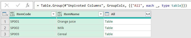
We will next group all repeated columns into their respective ItemCode and ItemName. To do this, we select both ItemCode and ItemName columns and go to the Transform Tab, where we select ‘Group By’. We name the new column ‘All’ and choose the operation ‘All Rows’ from dropdown list.
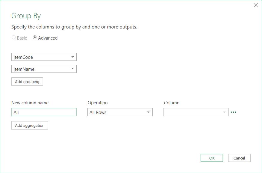
Once again, to keep the query dynamic we will replace the values {"ItemCode", "ItemName"} in the formula with GroupCols.
We are then going to add an index column in each table within the All column, such that when it reaches a row with new ItemCode and ItemName values, the index resets to one [1]. We then create a new blank step called Indexed and apply the following formula.
= Table.TransformColumns(#"Grouped Rows", {{"All", each Table.AddIndexColumn(_,"GroupIndex", 1, 1)}})
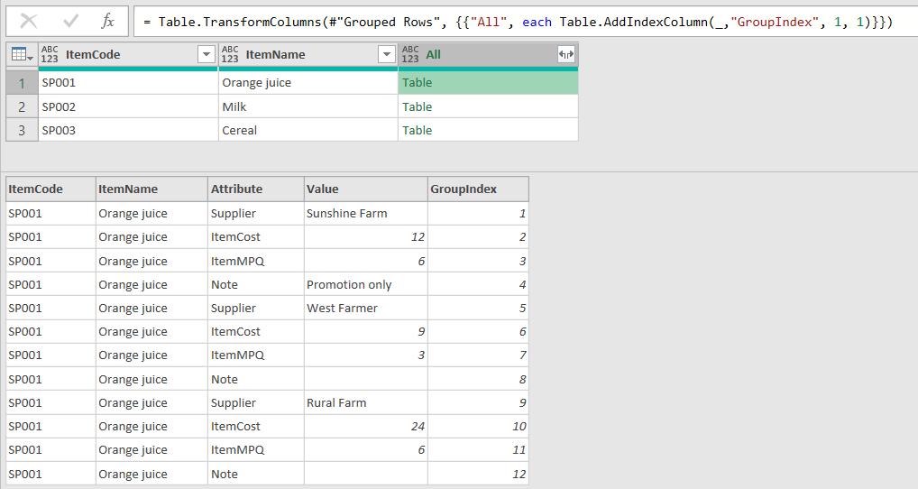
The above formula indexes the All column and is named GroupIndex, with the index starting at one [1] and increases in increments of one [1]. Next, we expand the All column which should then look like the following:
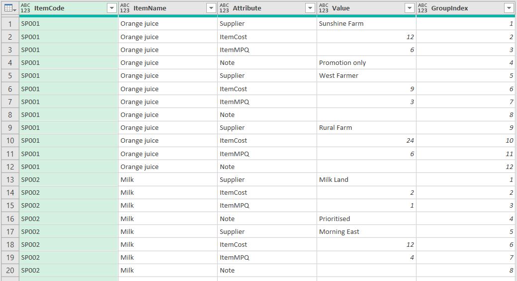
While the above indexing would allow us to separate the data based on each item code and name, we would like to further index and separate the data by suppliers as well. First, we need to establish the number of repeated columns or the number of rows per unique supplier which is four. To do this we use List.Count function as below:
=List.Count(Column)
We will rename this step as RepeatedCols, and next we use the following formula for a new blank step:
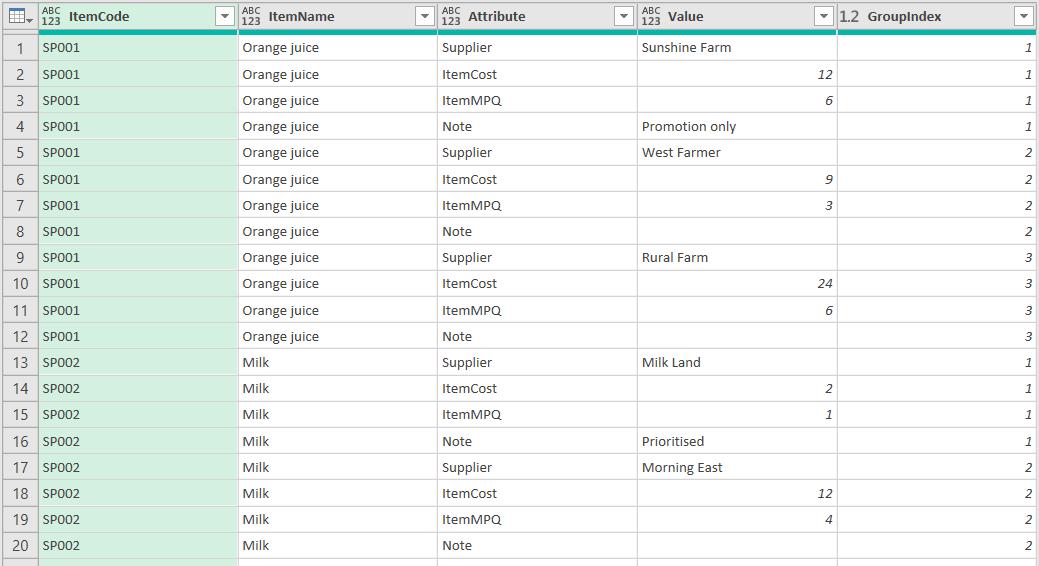
= Table.TransformColumns(#"Expanded All", {{"GroupIndex", each Number.RoundUp(_ / RepeatedCols), type number}})
The above formula rounds up the index column to the closest division of four, e.g. 1/4 = 0.25 rounded up is one [1], 2/4 = 0.5 rounded up is still one [1] etc. Thus, the query will now look like this:
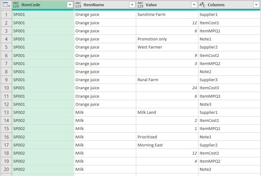
We next merge the Attribute and GroupIndex columns to give each supplier an index identifier using ‘Merge Columns’ under the Transform tab. We name the merged column as Columns.
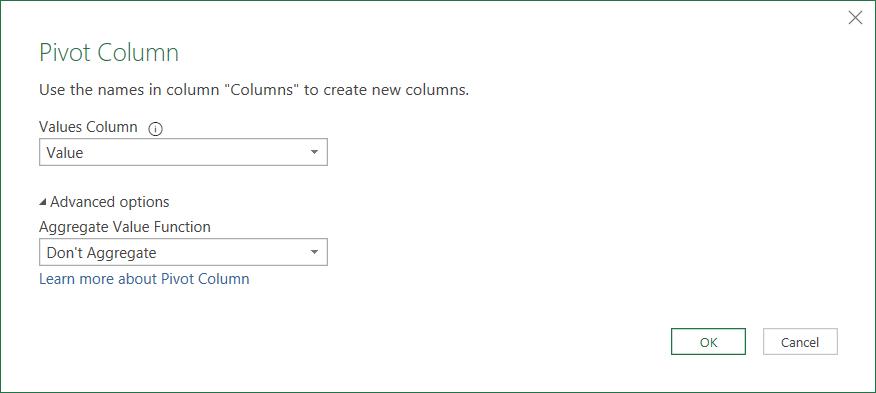
Then, we select the column Columns and click ‘Pivot Column’ under the Transform tab. We then choose the column Value as the ‘Values Column’ and click ‘Advanced options’ to select ‘Don’t Aggregate’ for the ‘Aggregate Value Function’.
Lastly, we convert “” back to null values using ‘Replace Values’, and finally, ‘Close & Load’. We should have the end result as follows:
It only takes two minutes if you were at 500 miles per hour!
The Final Friday Fix will return on Friday 27 May 2022 with a new Excel Challenge. In the meantime, please look out for the Daily Excel Tip on our home page and watch out for a new blog every business working day.