
Monday Morning Mulling: April 2020 Challenge
27 April 2020
On the final Friday of each month, we set an Excel problem for you to puzzle over for the weekend. On the Monday, we publish a solution. If you think there is an alternative answer, feel free to email us. We’ll feel free to ignore you.
Welcome to this month’s Monday Morning Mulling. If you thought this month’s challenge, seemed a bit week, you’re right – as there may be a bit of a week left over…
The Challenge
Imagine you have four years’ worth of daily sales (not all sales are displayed!):
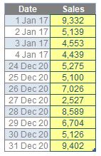
This month’s challenge was to prepare a monthly PivotTable summarising the sales monthly, allowing for one minor complication to add: each month’s sales reporting period ends on the final Friday of the month. Well, it is the Final Friday Fix! For example, Friday 24 April 2020 would be the final date of the April 2020 reporting period and Saturday 25 April would be the first day of the May 2020 reporting period.
We will use the Excel starter file to walk through our suggested solution.
Suggested Solution
This month’s problem could be solved simply using Excel – but our solution will use Power Query. We’ve done this for two reasons:
- It keeps the Excel file cleaner
- It allows the introduction of a very useful feature in Power Query that few seem to know about – Fill Up. But more on that shortly…
To begin, I will import the table (already called Sales_Data) into Get & Transform / Power Query.
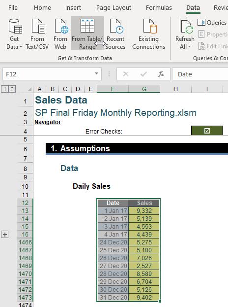
Here, having selected the Table, I have clicked on the Data tab in the Ribbon and clicked ‘From Table / Range’. This loads the Sales_Data into the Power Query Editor, viz.
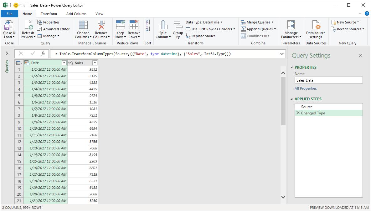
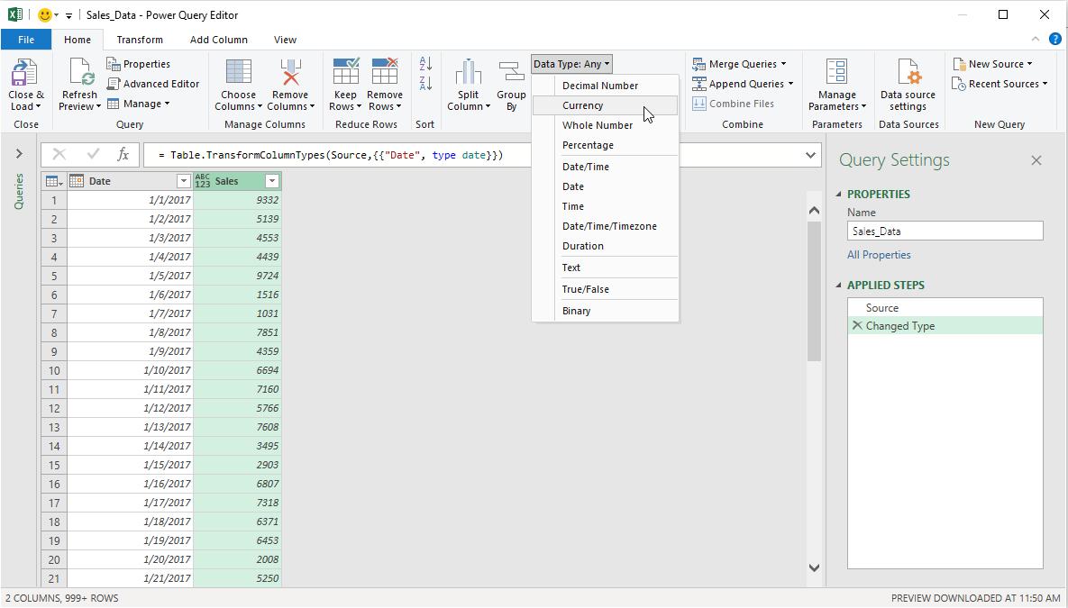
I remove the ‘Changed Type’ step automatically undertaken in ‘APPLIED STEPS’ and, instead, manually change the Data Types of the fields Date and Sales to Date and Currency respectively:
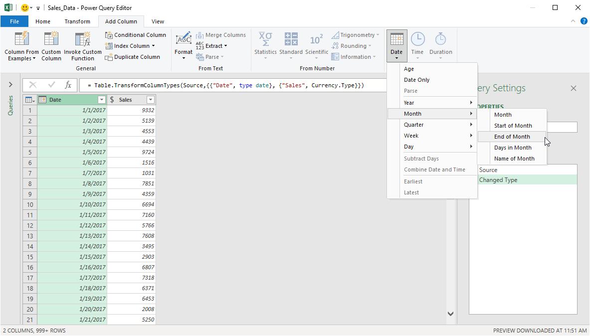
Now I will create a new column that will display the end of the month for each record – a bit like the formula =EOMONTH(Date,0) in Excel. To do this, I click back on the Date field, then from the ‘Add Column’ tab, I click on Date -> Month -> End of Month:
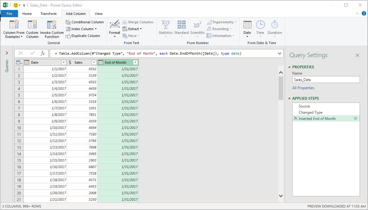
This gives me the end of the month for each sales record (already given the Date Data Type):
I want to subtract the Date from the End of Month, so that I can see how many days are left until the end of the month. Normally, I would use the Standard button in the ‘From Number’ section of the ‘Add Column’ tab, but it is greyed out since our Data Types are Dates, not numbers.
No matter: I shall have to write some very complex M code instead. On the ‘Add Column’ tab, I click the ‘Custom Column’ button in the General section and write the following:
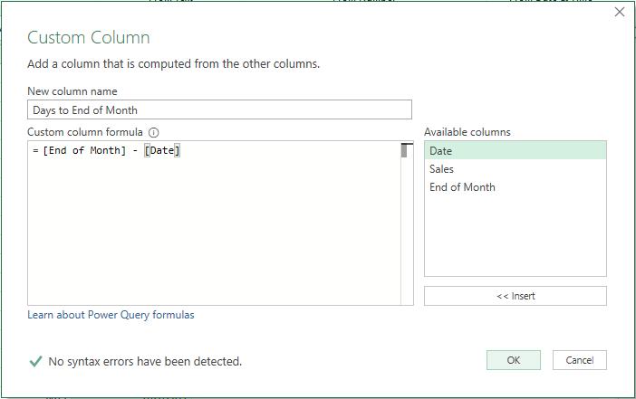
=[End of Month] – [Date]
Hopefully, you can follow that formula!
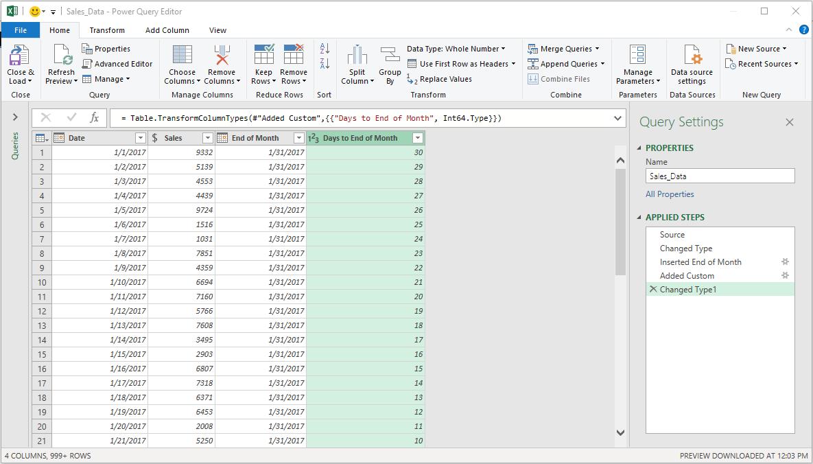
I change the resulting Days to End of Month field to a Whole Number Data Type, and I can immediately see how many days there are to the end of the month.
Now I have a plan:
- I need to add another field which identifies the day of the week
- I then add another Custom Column to flag the Fridays (one [1] for Friday, zero [0] otherwise)
- The final Friday will occur in the last week of each month, so when the Days to End of Month value is between zero (0) and six (6) inclusive. Therefore, I add a flag to highlight this last week (one [1] for record is in last week, zero [0] otherwise)
- Simply multiplying these last two flags together will show me the final Friday
- For this Final Friday flag, I simply replace the one [1] with the Date value at that point and replace all the zeroes [0] with null
- I then may Fill Up on this Reporting Month End date, which will be used to populate my PivotTable date.
Simple! All I have to do is, er, do it.
Step 1: Add Day of Week Identifier
This is a real toughie. Here, I simply click back on the Date field, then from the ‘Add Column’ tab, I click on Date -> Day -> Name of Day:
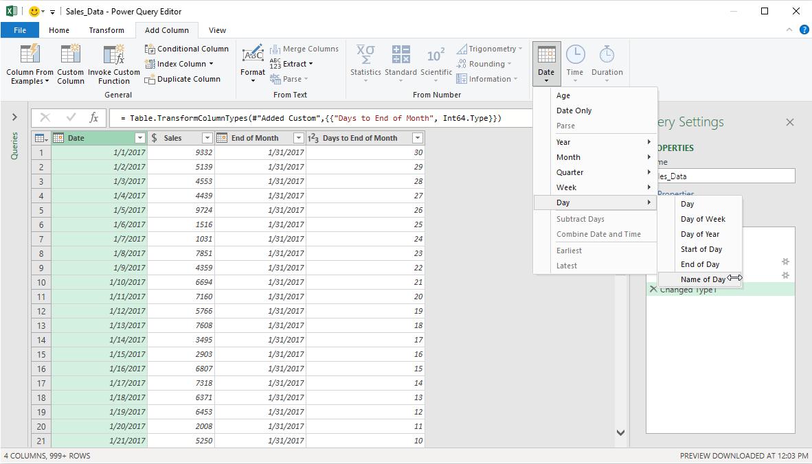
This gives me the new field Day Name, which is already given the Data Type Text, viz.
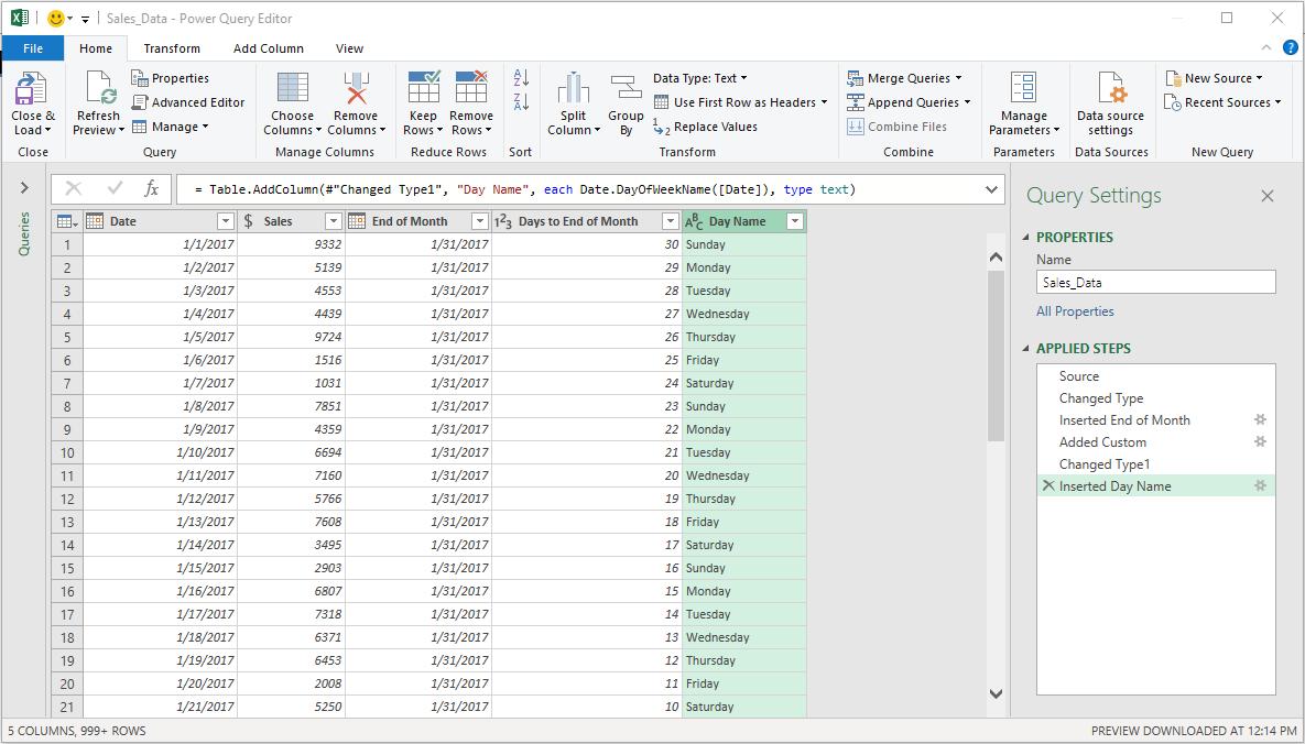
Step 2: Identify the Fridays using a Flag
This requires more nightmarish M code. Again, from the ‘Add Column’ tab, I click the ‘Custom Column’ button in the General section and write the following:
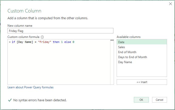
=if [Day Name] = “Friday” then 1 else 0
Alternatively, the same result could have been achieved by going to the ‘Add Column’ tab, but clicking on the ‘Conditional Column’ button instead:
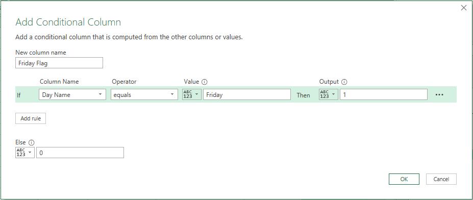
After changing the Friday Flag Data Type to Whole Number, we get:
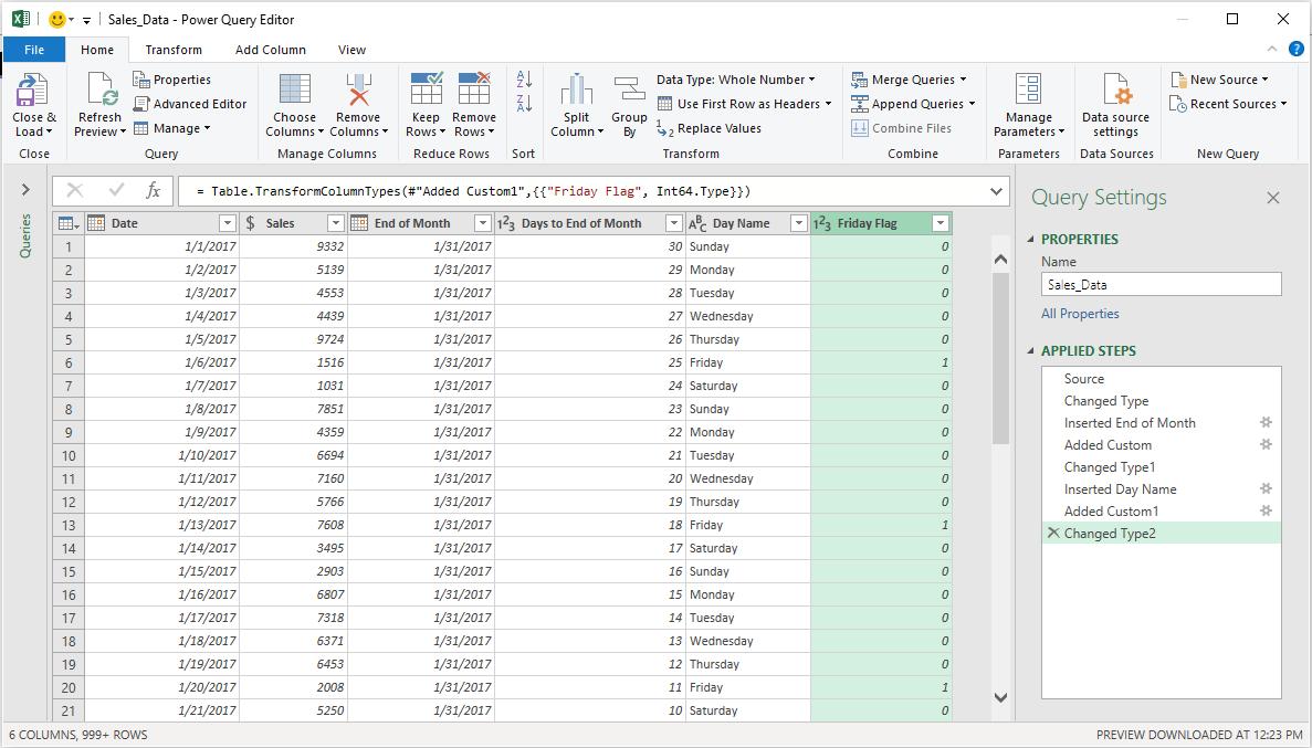
Each Friday displays a ‘1’ in the Friday Flag field, with all other dates showing zero. That’s just what we wanted.
Step 3: Create a Last Week Flag
This works similarly to the last step. I simply add another ‘Conditional Column’:
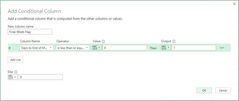
Here, if the value in the Days to End of Month field is less than or equal to six (6), then the Final Week Flag is one (1), else zero (0). Changing the Data Type of this flag to Whole Number as well yields the following:
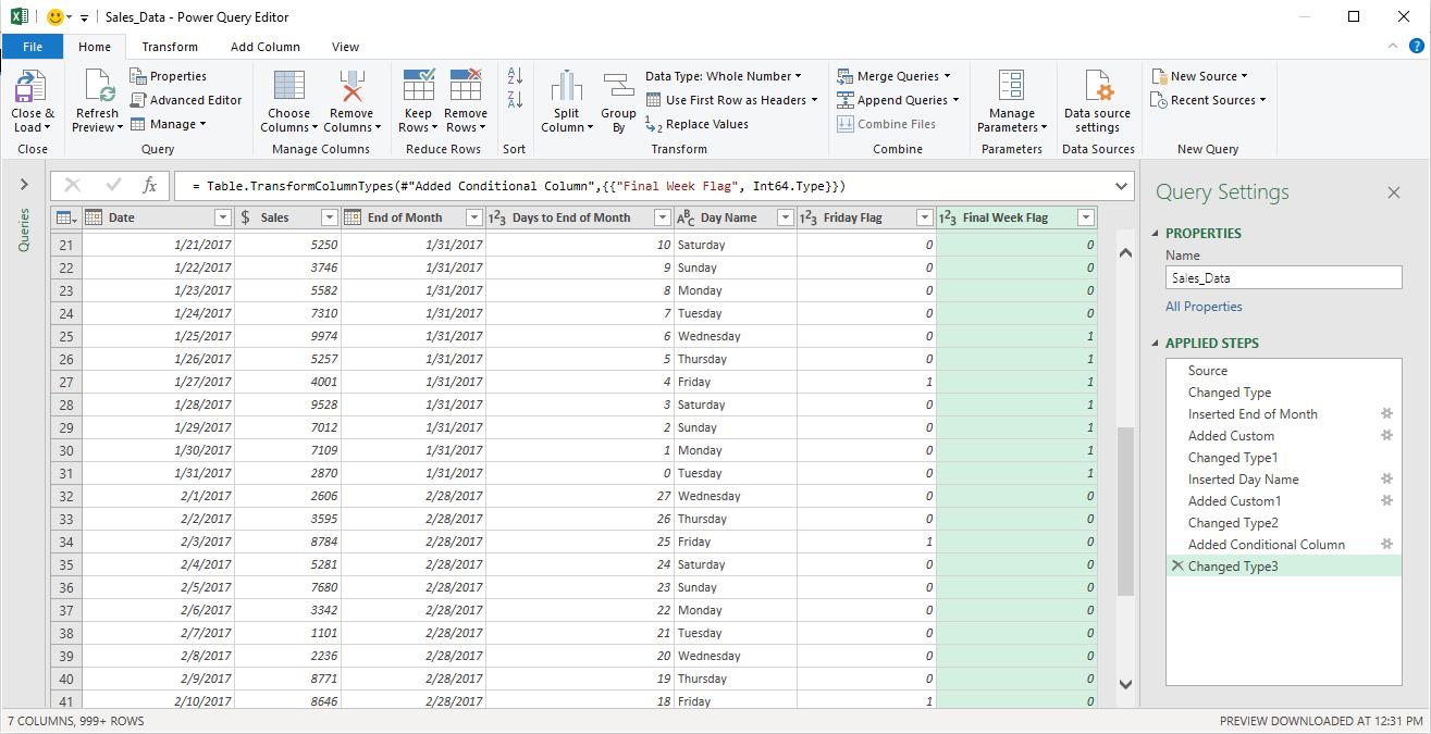
Some of you may have been wondering why I have been persevering with 1 and 0 rather than TRUE and FALSE. It’s because multiplication is trivial with numbers…
Step 4: Creating a Final Friday Flag
To reiterate, the final Friday is the Friday that occurs in the last week of the month. I already have a flag to identify each Friday, and another to denote the final week of each month. Given these are both Boolean flags [1, 0], all I need to do is multiply them together to generate my Final Friday Flag.
Multiplication is easy when the Data Types of both fields are numbers, which they are here. I simply highlight the Friday Flag and Final Week Flag fields and then select Multiply from the ‘Standard’ button dropdown on the ‘Add Column’ tab, viz.
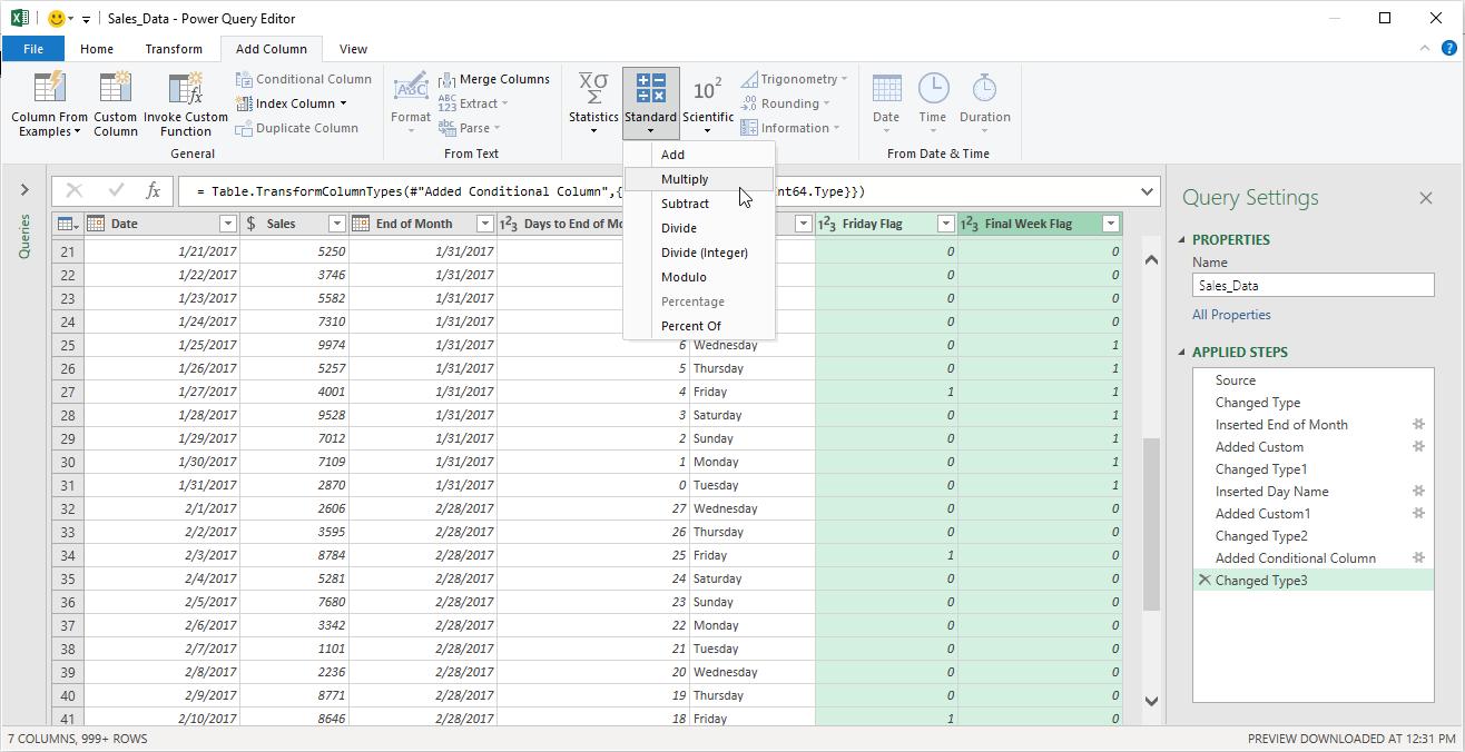
I then rename this Multiplication field Final Friday Flag:
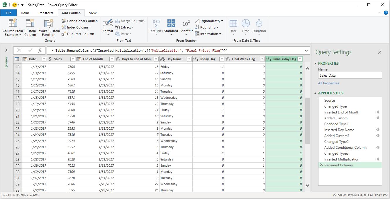
Due to what I do next, there is no need to change the Data Type yet…
Step 5: Replace the Final Friday Indicator with the Date
‘Replace Values’ will not work here, as this will substitute the same value on each occurrence of a one (1). This is not what we require: we want the date for that record to be used instead. This is still trivial using the ‘Conditional Column’ feature:
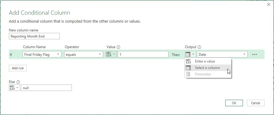
Using the ‘Add Conditional Column’ dialog, I am replacing each one (1) with the corresponding Date and making all other values null. Be careful here: the ‘Output’ field must select a column, not a value (see image above).
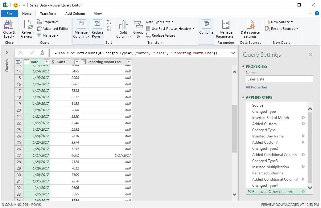
For this new field, Reporting Month End, I can change the Data Type to Date, and delete all the fields except for Date, Sales and Reporting Month End:
Step 6: Fill Up the Reporting Month End Dates
This Reporting Month End date is the date for all days prior to this final Friday. I need to Fill Up – and fortunately, Power Query has just the thing:
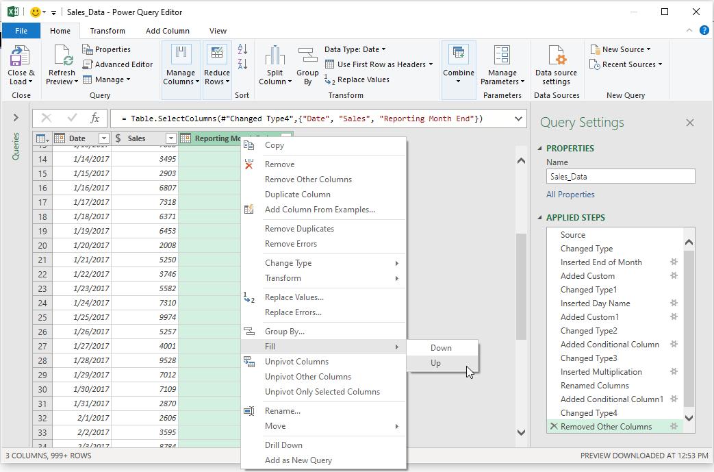
With the Reporting Month End field selected, I right-click and select Fill -> Up from the shortcut menus (as shown above). This is a seriously underestimated feature in Power Query, as you often need to cut off a selection by determining the end point. It is possible to do this in Excel, of course, but it usually requires offsetting or fiddling the ranges in the VLOOKUP, INDEX MATCH or XLOOKUP formulae, whereas this is quite a neat solution. That’s why I have used Power Query this month.
There is a little bit of tidying up to do, which includes avoiding a classic Power Query gotcha. Unless the final date in our Sales_Data table is the final Friday of a month, we will have some remaining null values in the Reporting Month End field. Using the dropdown filter may not appear to assist initially:

There appears to be no null. However, note the warning triangle: ‘List may be incomplete’. Remember to ‘Load more’ and then de-select null:

Finally, using the Reporting Month End field (not the Date field), I would add the Reporting Month (Date -> Month -> Month Name), the Reporting Month Number (Date -> Month -> Month) and the Reporting Year (Date -> Year -> Year) as additional columns, using the ‘Date’ button on the ‘Add Column’ tab:
Date -> Month -> Month
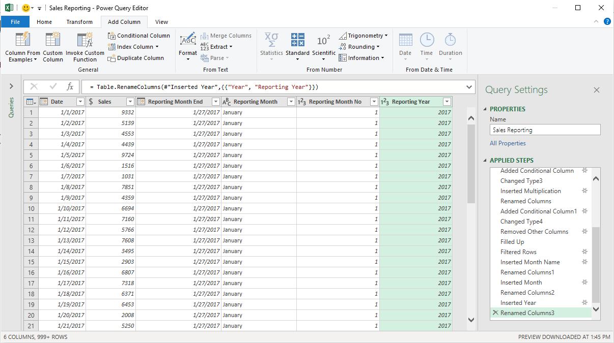
Renaming the query ‘Sales Reporting’, I then ‘Close and Load To…’:
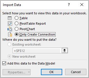
I only create a connection (no need to display this Table), but it is important that I ‘Add this data to the Data Model’. This is so this Table may be accessed in Power Pivot:
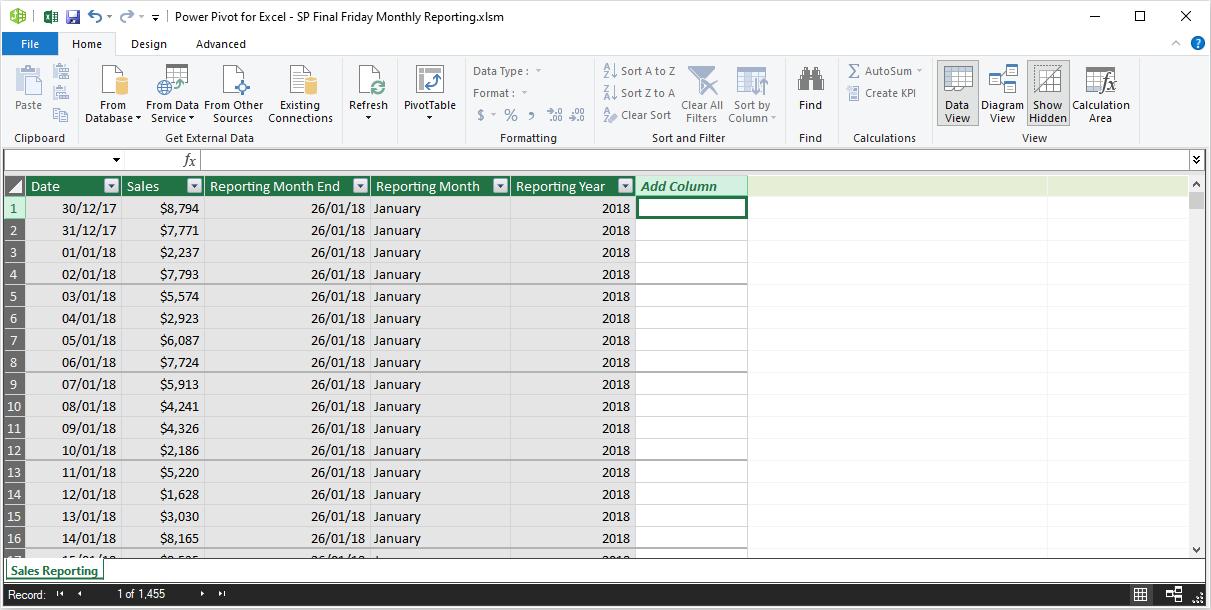
You may wish to change the formatting (something you cannot do in Power Query).
One more thing: given we don’t want the Reporting Month to be displayed alphanumerically, we need to sort the Reporting Month by the Reporting Month No. This is easily managed, by clicking the ‘Sort by Column’ button on the Home tab:
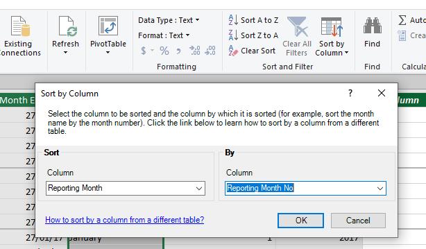
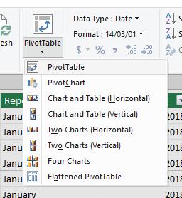
Once satisfied, from the Home tab, I can insert a PivotTable:
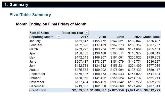
And there you have it: one PivotTable with the sales summarised by Reporting Month, where each reporting ends on the final Friday of that month.
Check out the attached Excel file for our suggested solution.
The Final Friday Fix will return on Friday 29 May with a new Excel Challenge. In the meantime, please look out for the Daily Excel Tip on our home page and watch out for a new blog every business workday.