
Monday Morning Mulling: March 2023 Challenge
3 April 2023
On the final Friday of each month, we set an Excel / Power Pivot / Power Query / Power BI problem for you to puzzle over for the weekend. On the Monday, we publish a solution. If you think there is an alternative answer, feel free to email us. We’ll feel free to ignore you.
The challenge this month was to transform data into a useful Table. Did you succeed?
The Challenge
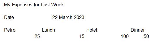
This month, we had a Power Query challenge. We received some expense information in an Excel workbook which is not in a format that is compatible with our usual layout.
You can download the original challenge file here.
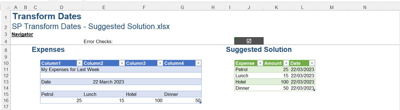
Therefore, this month’s challenge was to extract the data from a sheet in the supplied Excel workbook and present it in a Table that can be appended to other expense data. The result should look like the Table below:
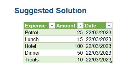
Note: Our dates are in UK format – this was not part of the challenge!
As always, there were some conditions:
- this is a Power Query challenge: no Excel formulae allowed
- the solution should allow us to add more expenses
- the solution should need less than 10 steps (one transformation per step)
- All the steps can be achieved using the User Interface (UI) from one query. No M code is needed.
Suggested Solution
You can find our Excel file here which demonstrates our suggested solution.
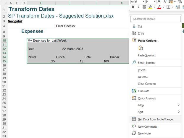
We start by extracting the data. We can select the data and right-click to ‘Get Data from Table/Range’. This will also convert our data into a Table:
This gives us a query, which we rename to Expenses:
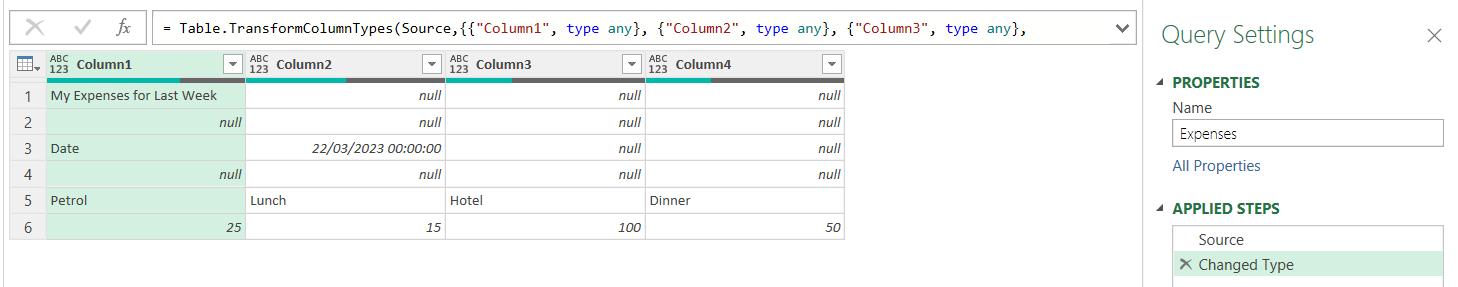
The ‘Changed Type’ step has not achieved anything as our data is currently mixed in the columns. We can remove this step.
We have two tasks. We need to extract the date, and we need to format the expenses. We start by extracting the date: we right-click on the cell containing the date:
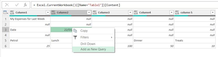
We choose ‘Add as New Query’ which creates a query called Column2 with only two [2] steps:
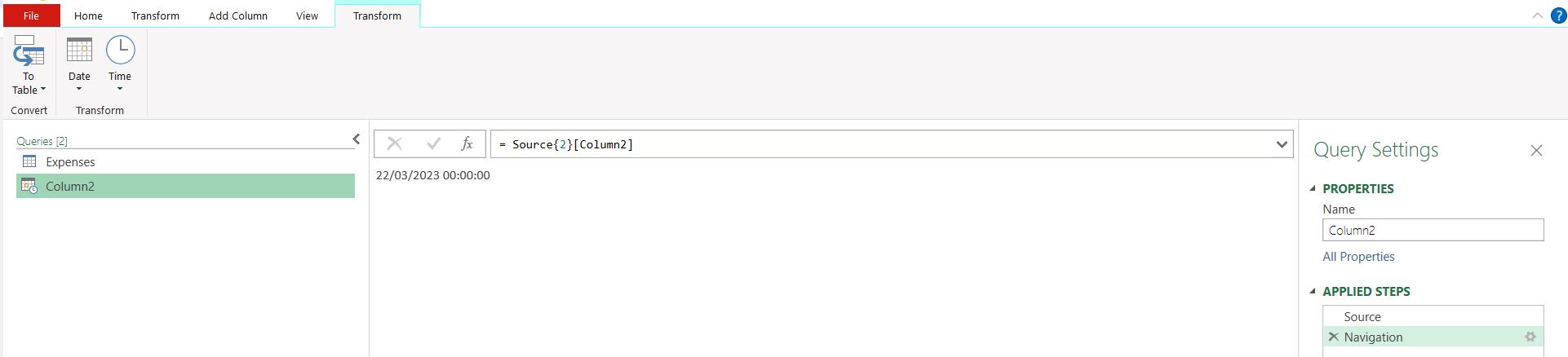
We didn’t say we couldn’t create another query, only that all the steps had to be created from one query! [Cheat, cheat – Ed.]
In the Expenses query, we choose ‘Keep Rows’ and then ‘Keep Bottom Rows’ from the Home tab.
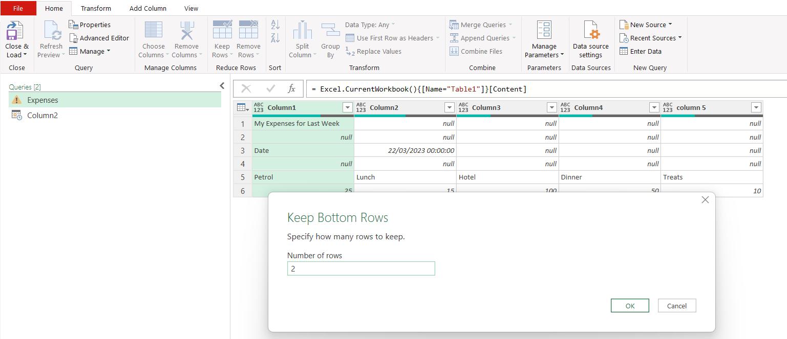
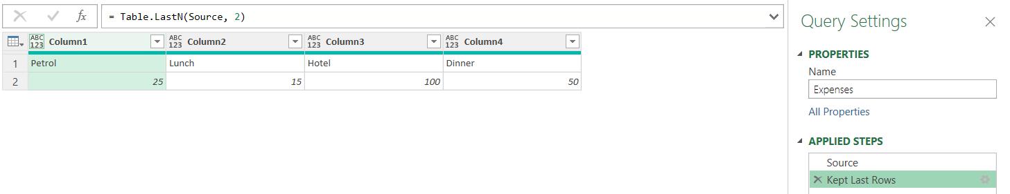
We choose to keep two [2] rows. This leaves us with the expense data:
We choose ‘Use first row as headers’ from the Home tab:
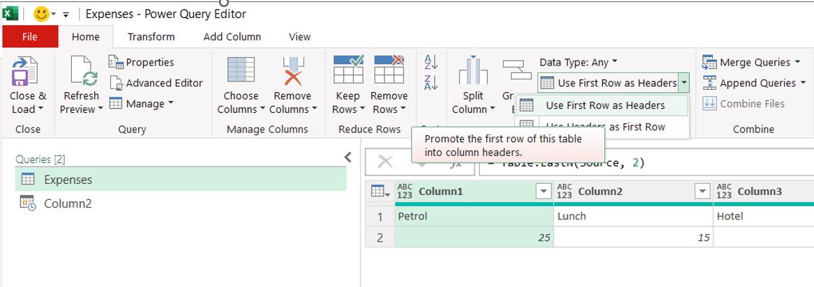
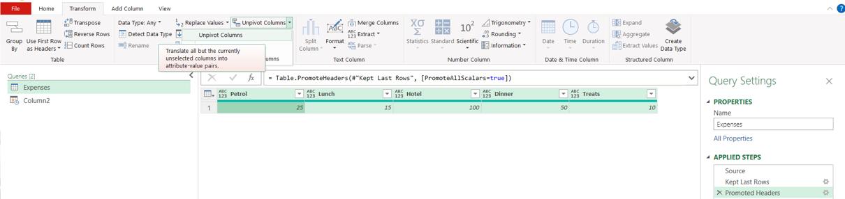
This generates a ‘Changed Type’ step, which we delete as we are about to select all the data and ‘Unpivot Columns’ from the Transform tab:
Now, we can add the date by using ‘Custom Column’ from the ‘Add Column’ tab:
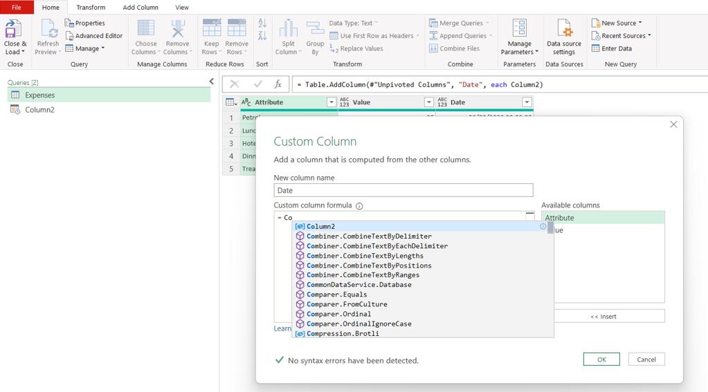
We choose the Column2 query and create the new column Date.
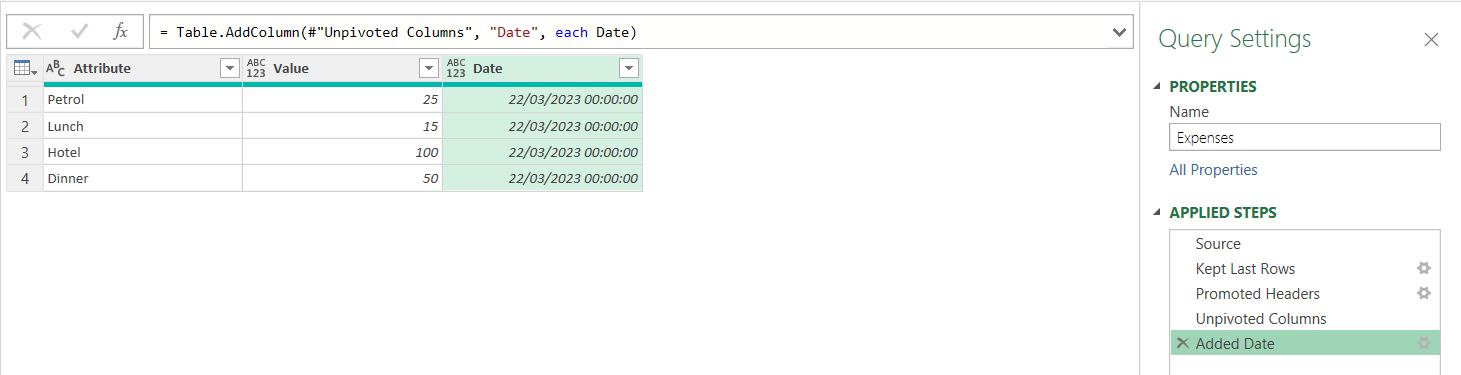
Now we just need to tidy up. We rename the columns and assign the correct data types:
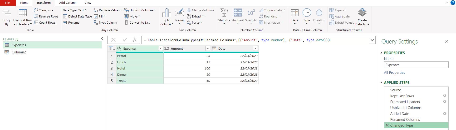
We have our solution in nine [9] steps!
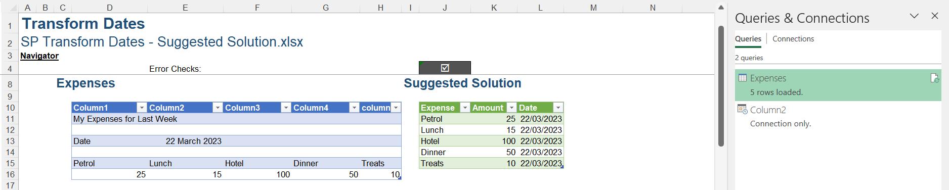
We choose ‘Close & Load To…’ from the Home tab so that we can put Expenses on the same sheet as the data, and keep Column2 as a ‘Connection Only’ query:
Finally, we show that more expenses can be added:
The Final Friday Fix will return on Friday 28 April 2023 with a new Excel Challenge. In the meantime, please look out for the Daily Excel Tip on our home page and watch out for a new blog every business working day.