
Charts and Dashboards: Data Tables - Part 2
3 June 2022
Welcome back to our Charts and Dashboards blog series. This week, we’ll go step-by-step through the process of constructing a one-dimensional Data Table.
Last week, we looked at the below example of a 1-D Data
Table:
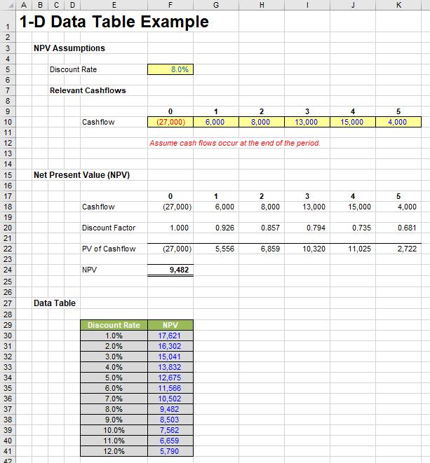
It is actually very easy to construct a table (a Data Table) similar to the one displayed in cells E29:F41 above. The required discount rates are simply typed into cells E30:E41, but the heading in cell F29 is not what it seems.
For a 1-D Data Table to work using a columnar table similar to the one illustrated, the top row of the second and any subsequent columns have to contain the reference to the output cell(s). Many modellers will do this, putting the headings in the row above instead and then they may or may not hide this row in order to compensate.
There is a crafty alternative (employed above). Using CTRL + 1, ALT + H + O + E or selecting ‘Format Cells…’ from the Format drop-down in the Cells grouping of the Home tab of the Ribbon to Format Cells. Then, if we go to the ‘Number’ tab we can still type the formula(e) in but change the outward appearance of the cell(s). It is with this borne in mind that cell F29 is formatted as follows:
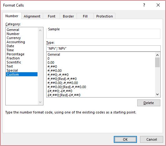
Here, I have typed in ““NPV”;”NPV””. Essentially, what this does here is replace all non-negative numbers with the text “NPV” and negative numbers with the text “NPV”. You might wonder why we have typed this in twice? If the number is negative and the second “NPV” has not been defined the negative number would be replaced by “-NPV” instead – which is not what we want.
Once this formatting has been applied and the formula
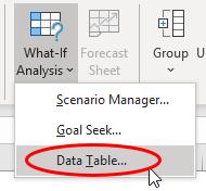
=F24
has been typed into the header in cell F29 (taking on the appearance “NPV”), then select cells E29:F41and go to ‘Data Table…’ in the What-If Analysis drop-down list in the Forecast grouping of the Data tab on the ribbon (Alt + A + W + T):
This calls the ‘Data Table’ dialog box:
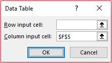
At this point, confusion often sets in as users are often unsure whether they should be entering details in the ‘Row input cell:’ and / or ‘Column input cell:’ input boxes. The rules are very simple:
- Referenced directly, the inputs and outputs must be on the same sheet as the Data Table (although there are ways and means around this which we’ll cover in a few blogs’ time)
- Use only one input box if you want to flex one input; use both if you wish to flex two
- If inputs are in a column in the Data Table, use the ‘Column input cell:’ input box
- If inputs are in a row in the Data Table, use the ‘Row input cell:’ input box.
Here, inputs are in a column and we want to use them to substitute for the value in cell F5 so, we select cell F5 for the ‘Column input cell:’ input box. Clicking ‘OK’ results in the following summary:
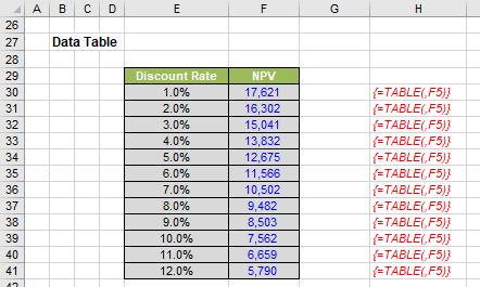
That’s it – you have your “What-if?” analysis. It should be noted that at this point you may not enter any rows or columns into the Data Table (or delete any either). This is because the formula
{=TABLE(,F5)}
has been entered into cells F30:F41. The braces (‘{‘ and ‘}’) may not be typed in. These are special characters created by Excel when you type the formula
=TABLE(,F5)
and press CTRL + SHIFT + ENTER rather than ENTER. This is known as an array formula and these cannot be edited, merely deleted in their entirety.
If the table had been across a row instead, ensure that the input values are in the top row, and that the ‘headings’ are in the first column (that is, transpose the example table, above). Then, you would populate the ‘Row input cell:’ box instead.
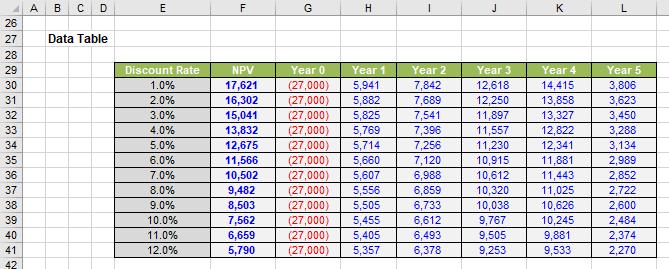
1-D Data Tables do not need to be simply two columns or two rows. It is entirely possible to display the effects on more than one output at the same time provided you wish to use the same inputs throughout the sensitivity analysis as follows:
Sometimes, you may find all of the numbers in your Data Table are identical. If this happens, you need to check your calculation settings. To do this, go to Excel Options (File -> Options orALT + F + T) and then select ‘Formulas’. In the ‘Calculation options’ section, ensure the ‘Workbook Calculation’ is set to ‘Automatic’:
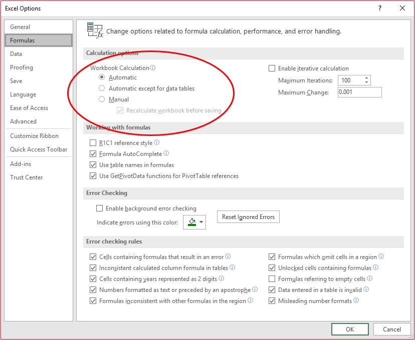
Any other setting will not calculate Data Tables correctly. The reason for this is Data Tables can consume a significant amount of memory and slow down workbook calculations – hence the options to disable them.
Next week we’ll cover two-dimensional Data Tables.
That’s it for this week. Come back next week for more Charts and Dashboards tips.