Charts and Dashboards: Charting Example – Extended Case Study Part 6

Welcome back to our Charts and Dashboards blog series.  This week, we’re going to continue to look at the example chart and finally cover the workings behind it.

We’ve now covered almost every part of our variable chart.  Let’s look at the workings behind the graphed data.

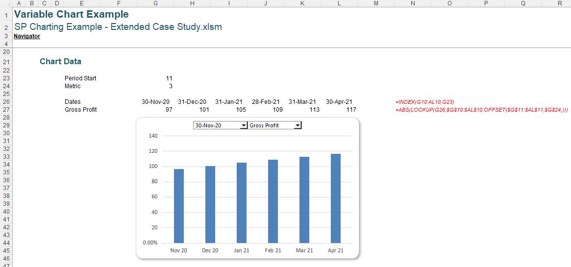
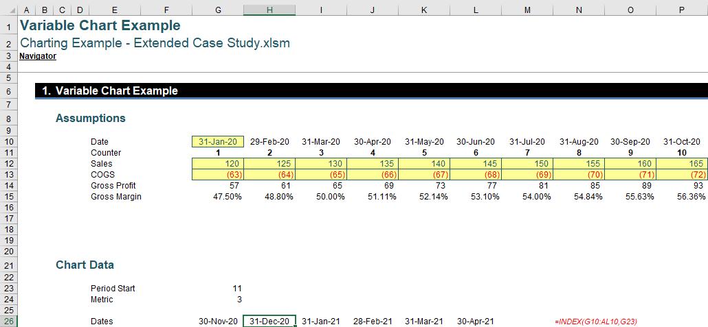
Rows 26 and 27 contain the lines of data actually linked to our graph.

We have designed the formulae in these lines to display the data as selected in the Combo Boxes.  Let’s take a look at the Dates first.  Cell G26 contains the following formula:

This will select the value in our dates list in the position specified in G23, as G23 is the Cell link for our Period Start Combo Box.  This will return the value specified in the Combo Box.  Subsequent cells in this row contain the following formula:

This will calculate the final date of the month one month after the date in the cell to the left.

Row 27 is more complex.  To start, the heading (E27) is actually a formula:

This will return the value in our list of headings above in the position specified in G24, as G24 is the Cell Link for our Metric Combo Box, this will be the value specified in the Combo Box.  This has been done to create a dynamic heading that updates to reflect the data presented here.

On to the data itself, let’s take a look at the formula in G27:

This one is a little more complicated, so let’s work backwards. 

The OFFSET function here takes the reference of G11:A11, and then returns the range that is a number of rows beneath the initial reference equal to the number in G24.  In this instance, with COGS selected in the Combo Box, the Cell link (G24) will return two [2], as COGS is the second value in the list.  This will “offset” G11:A11 two rows down, returning the row containing the COGS data (G13:A13).

The LOOKUP function will look up the value in G26 (the date to be graphed) in the range G10:AL10 (the date headings for the data), and then return the value in the third argument (OFFSET($G$11:$AL$11,$G$24,), which in this instance evaluates to G13:A13) in the same position as G26 is in G10:AL10, effectively looking up the selected Metric’s value within the period stipulated in the Combo Box.  The reason behind using the LOOKUP function here over other similar functions is so that we can deal with the scenario where the final date is selected:

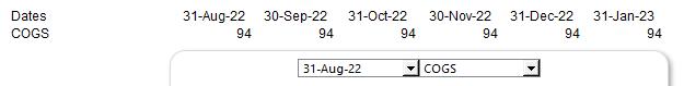
Here we have selected 31-Aug-22 within the Combo Box.  This is the final date that data has been provided for, and as such the LOOKUP function will not be able to find the subsequent dates within the data range.  In this scenario, the LOOKUP function defaults to using the final value of the data, which is the desired treatment here (this is because LOOKUP searches for the largest value less than or equal to what you are looking for, needing the lookup data to be in ascending order, which dates always are).

Finally, the whole formula is wrapped in an ABS function, leading to the absolute (non-negative) value being produced.  This will prevent negative values from pulling through, which allows us to display COGS as a positive number which is easier to understand.

There we have it: a graph that can display various metrics covering various dates, customisable by Combo Boxes.

That’s it for this week.  Come back next week for more Charts and Dashboards tips.