Charts and Dashboards: Charting Example – Extended Case Study Part 4

Welcome back to our Charts and Dashboards blog series.  This week, we’re going to continue to look at the chart example, and begin to consider how it is actually constructed.

We’ve looked at the assumptions and formatting surrounding our chart.  Now let’s look at how it’s constructed.

We’ve used Combo Boxes to allow users to select the start date of the graph and the metric to graph, making the selection within the graph area.  To insert a combo box, you must first navigate to the Developer tab in the Ribbon.

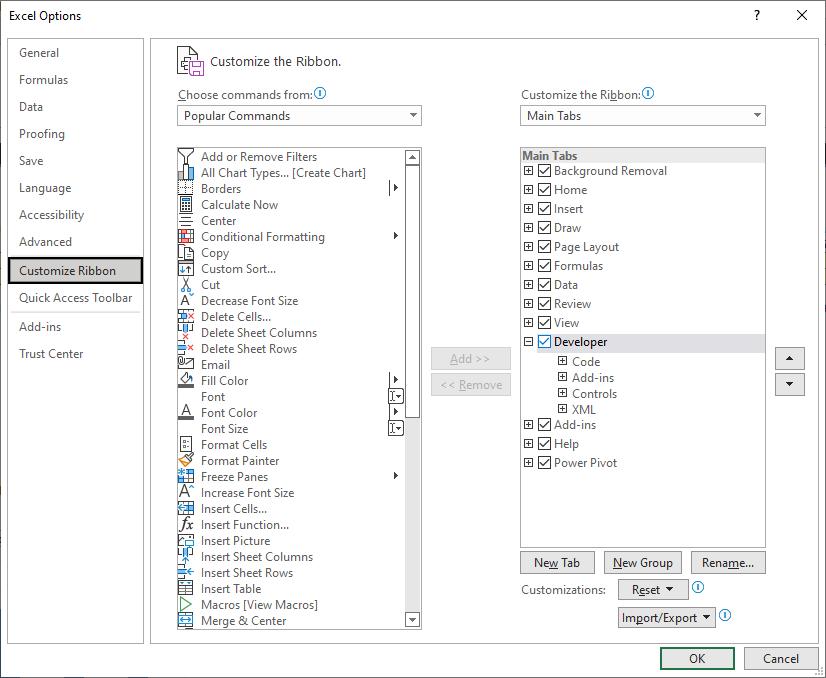
If you do not see the Developer tab, then you will need to enable this.  This may be done within Excel’s settings.  Navigate to File and click on Options.  This will open up the 'Excel Options' window.  From here, you must click on ‘Customize Ribbon’ on the left and then tick Developer within the menu on the right:

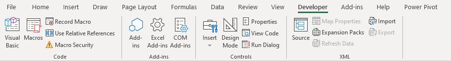
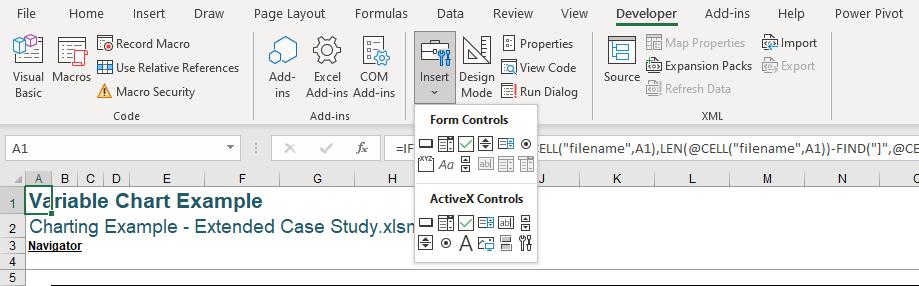
From the Developer tab, within the Insert menu we can see the kind of controls that can be inserted.  We are interested in the Form Controls, as these can be linked to a cell.  The ActiveX Controls require the use of VBA, so to keep it simple, we have stuck with Form Controls in this instance.  The Combo Boxes that we have used are the second choice on the first row in this list.

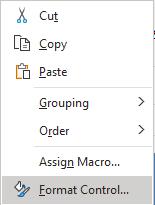
When the Combo Box is first inserted, it will not do anything.  It needs to be linked up both to a cell and to a list of values.  To do this we right-click on it and select ‘Format Control...’.

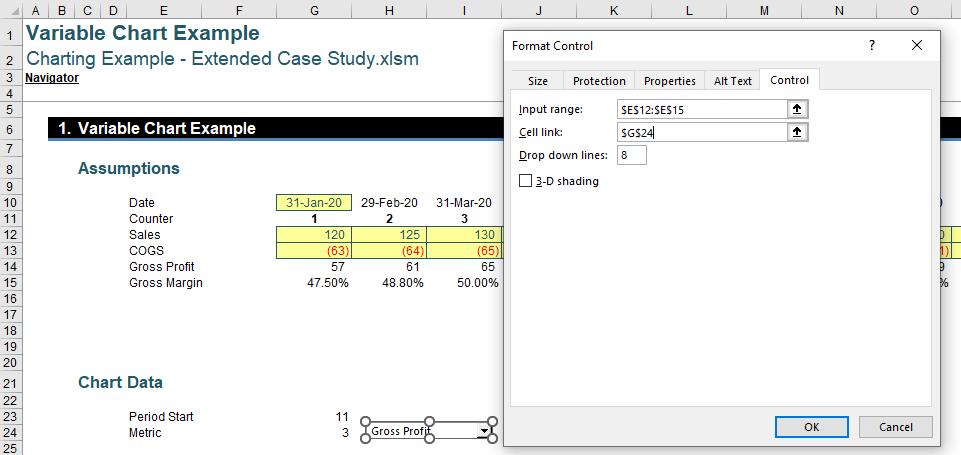
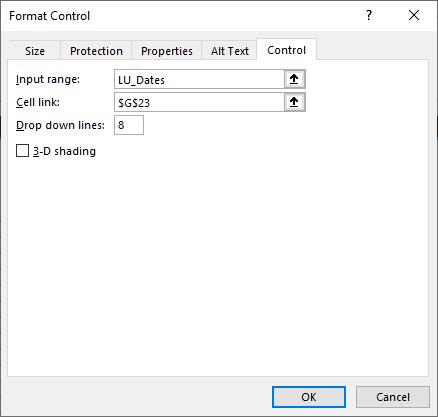
Navigating to the Control tab of this option menu allows us to choose the Input range and Cell link.  If you do not see the Control tab, you will have inadvertently inserted an ActiveX control (just delete it and start again).

The Input range is the list of variables that can populate the Combo Box.  For this one, we have chosen cells E12:E15, being the cells that contain the headings of the metrics that we will graph.  This list must be vertical (horizontal source data only recognises the first cell in the range).  We must also choose a Cell link, which is the cell linked to the Combo Box, updating to contain a numerical value equal to the position in the list of the value selected.  Here, we have chosen G24 for this Combo Box.  This is a two-way link, meaning that if the value in the linked cell is updated manually, the selection in the Combo Box will automatically change to reflect this.  The Drop down lines option simply defines the maximum number of options to show when the drop down arrow is clicked within the Combo Box, before you will need to scroll to view more.

We will also want to create a Combo Box where the starting period can be selected.  If we follow similar steps to above, choosing cell G23 as the Cell link, it may be tempting to choose G10:AL10 as our input range.

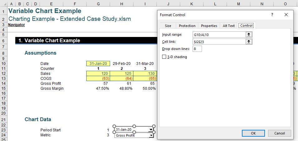
However, as mentioned above, the Input range must be vertical, selecting this horizontal list of dates will mean that only the first date can be selected.

To fix this, we must transpose our list of dates from a horizontal list to a vertical list.  This may be performed by making use of a counter and the OFFSET function.

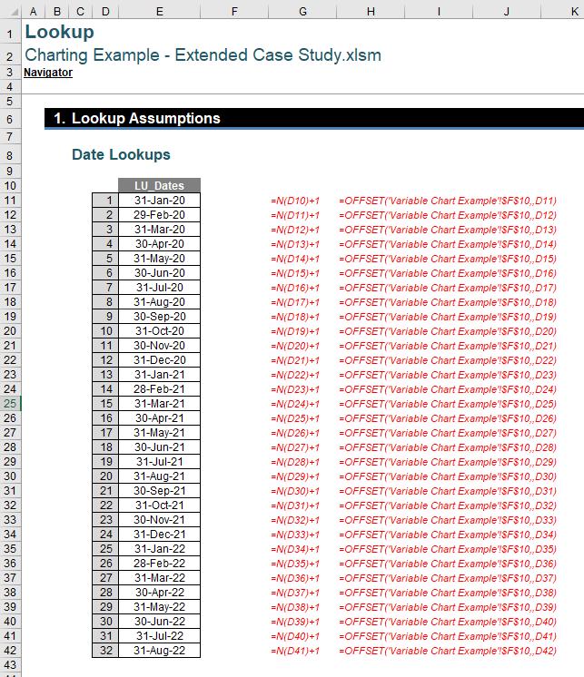
We have created a counter in column D using the N function:

This formula will take the numerical value of the cell above and then add one [1] to it.

We then use the OFFSET function.

OFFSET Reminder

OFFSET employs the following syntax:

The arguments in square brackets (height and width) can be omitted from the formula.  Most commonly, OFFSET(reference, rows, columns) is employed to select a reference rows rows down (-rows would be rows rows up) and columns columns to the right (-columns would be columns columns to the left) of the reference.  For example, consider the following grid:

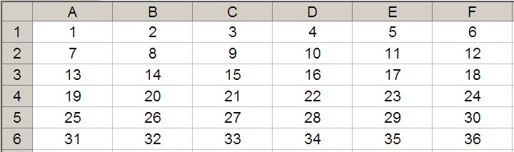
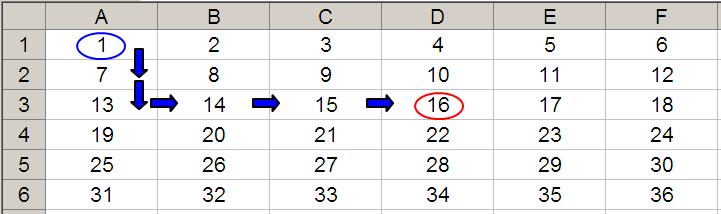
OFFSET(A1,2,3) would take us two rows down and three columns across to cell D3.  Therefore, OFFSET(A1,2,3) = 16, viz.

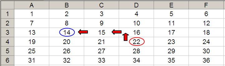
OFFSET(D4,-1,-2) would take us one row up and two rows to the left to cell B3.  Therefore, OFFSET(D4,-1,-2) = 14, viz.

Back to Our Example

The formula in cell E11 is given by

This formula will look a number of cells to the right of 'Variable Chart Example'!$F$10 (the cell before the start of our date range) equal to the counter, essentially transposing our date ranges.

We have given this list of dates a Range Name of LU_Dates to make referring to it more straightforward (LU stands for “Look Up”).  We may now choose to use LU_Dates as the Input range.

As this list is vertical, the Combo Box will now work as intended.

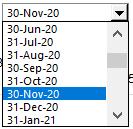
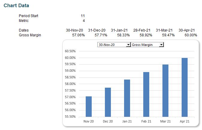
We can now select our Period Start and Metric from these Combo Boxes and watch cells G23 and G24 in line with our choices.

That’s it for this week.  Come back next week for more Charts and Dashboards tips.