
Charts and Dashboards: Interactive Charts – Part 1: Form Controls
24 July 2020
Welcome back to this week’s Charts and Dashboards blog series. Over the next few weeks, we’ll talk about interactive charts. This week, we will consider Form Controls and how to create Check Boxes using them.
Excel offers a lot of options to interact with charts, one of which is Form Controls. With Form Controls, we can add a data selection option to charts, such as a Check Box or a Drop-down List.
Let’s consider an example. To create Check Boxes for a chart, one option might be to create a linked duplicate table of the original data.
We create a row for Check Box value TRUE or FALSE. In each cell of the data, we apply a condition that if the Check Box shows FALSE, it will return #N/A error, otherwise, it will return the original value. The reason for using the NA() function rather than returning a zero or blank cell is that cells with #N/A will not be displayed in line charts, while cells with zero or blank will still be shown, as a straight line at the bottom of the chart. However, for a column chart, this would not have the same impact.
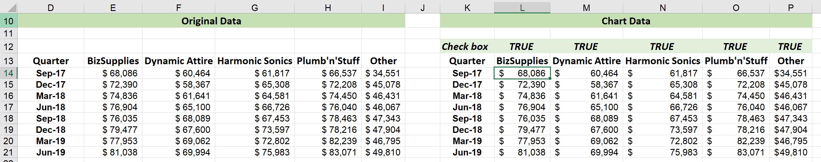
A suitable formula for cell L14 might be:
=IF(L$12,E14,NA())
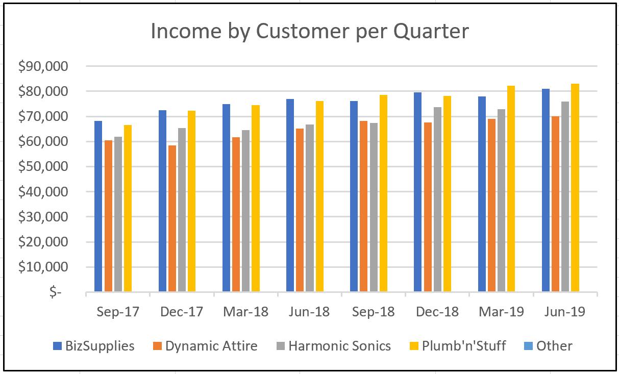
Next, we will insert a column chart based on the Chart Data:
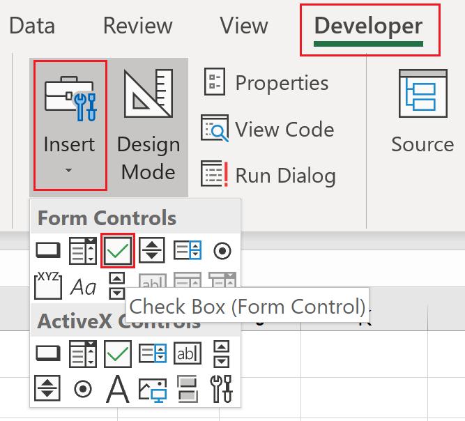
In order to create Check Boxes for this chart, go to the Developer tab on the Ribbon (you may need to display it first using File -> Options -> Customize Ribbon), and below the Insert menu, choose the ‘Check Box’ icon:
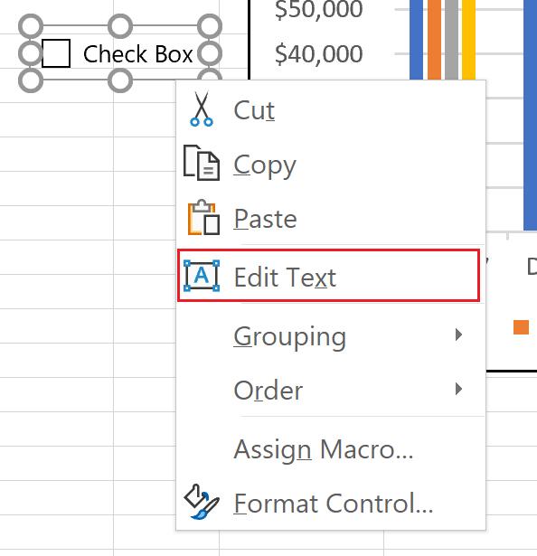
We will drag and drop the icon on to the worksheet. We may rename this Check Box by right-clicking on the Check Box and choosing ‘Edit Text’:
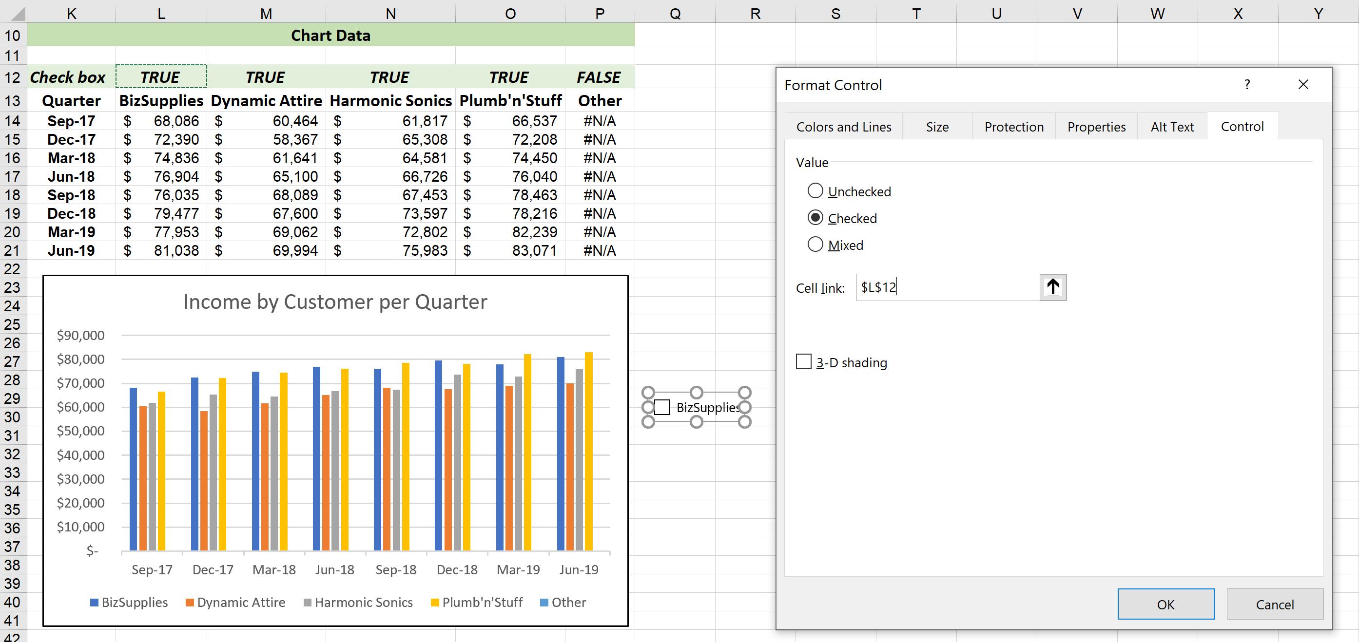
Now, we have to set up a control by right-clicking on the Check Box, choosing ‘Format Control’. A dialog will appear. On the final tab, Control, choose Checked, and choose ‘Cell link’ at the Check Box row according to the cell being referred to (e.g. for BizSupplies, we would select L12). The Check Box returns TRUE in the Cell Link cell when checked, and FALSE when unchecked.
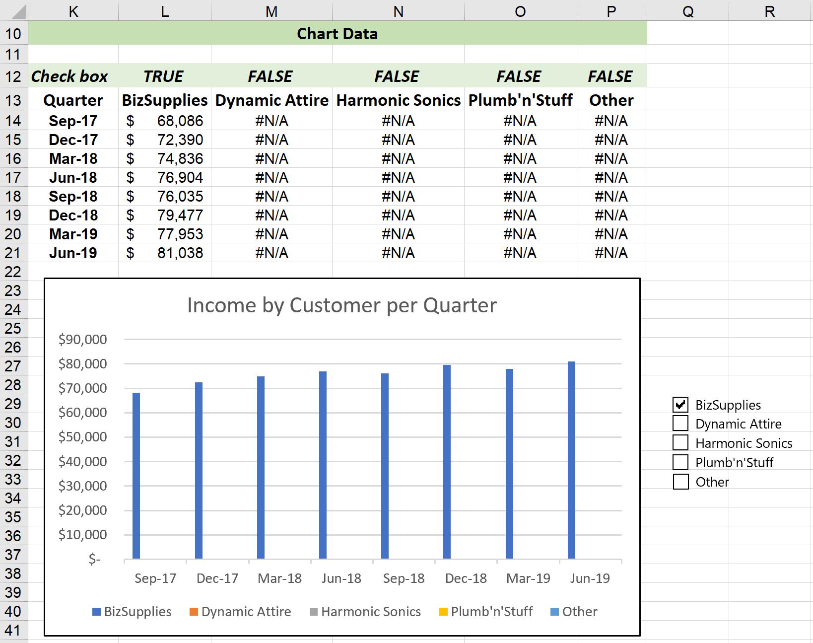
We will do the same for the rest of the Check Boxes. After inserting Check Boxes for all of the fields, we may perform a test. Below, if we check the BizSupplies box only, in the chart, only the BizSupplies data will be shown. In the Chart Data, the Check Box cell for BizSupplies will also show TRUE. The remaining references will still display FALSE. As a consequence, their corresponding data will be displayed as #N/A, meaning there will be no corresponding lines or columns shown on the chart.
Now, we need to create the Check Boxes on the chart legend. Right-click on the Check Boxes and a ‘Drawing Tools, Format’ tab will appear on the Ribbon. Here, we may choose the shape fills, outlines and effects as we wish.
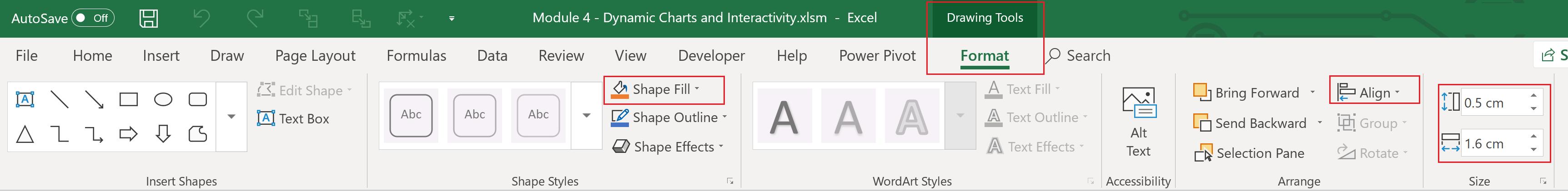
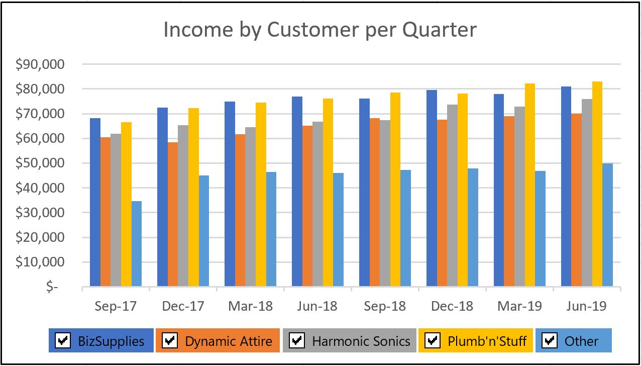
Particularly in this example, we choose the shape fill with matching colour for each Check Box (one tip is that you can apply RGB number so that the colours are exactly matched). Then we drag the Check Box to overwrite the existing legends, then adjust their height and alignment, so that the interaction looks much better:
That’s it for this week, check back next week for more Charts and Dashboards tips.