Charts and Dashboards: Conditional Chart Labelling – Part 1

Welcome back to our Charts and Dashboards blog series. This week, I take the first step towards creating conditional chart labels by producing multiple number formats.

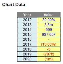
I have the following chart data:

“All” I have to do is create the associated Excel chart with replicated label formatting:

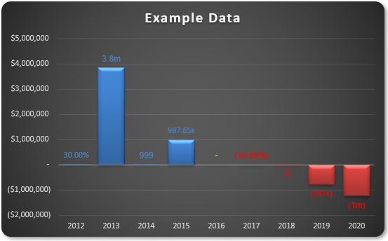
Do you see the need for supposed conditional formatting in the chart? I require positive values to be blue, zeros to be yellow and negative values to be in red – both labels and fill colours. It is possible, but I need to break the task down into various steps.

Essentially, there are several steps:

1. Understand how I can create multiple number formats in Excel, never mind in a chart data label
2. Create the basic chart
3. Create the formatting in the data labels, realising custom number formatting will not work and conditional formatting may not be applied
4. Make the solution robust enough to cope with saving the file and re-opening.

I will address all four areas, as I try to create the appearance of conditional formatting, but this week I will concentrate on step 1.

Step 1: Creating Multiple Number Formats in Excel

This is more a challenge of understanding how it works, rather than trying to solve the problem from scratch, as the inputs have already been formatted accordingly.

Returning to my problem, the data appears as follows:

Here, the correct custom formatting has been generated for numbers simply typed in, without using VBA code or Excel formulae.

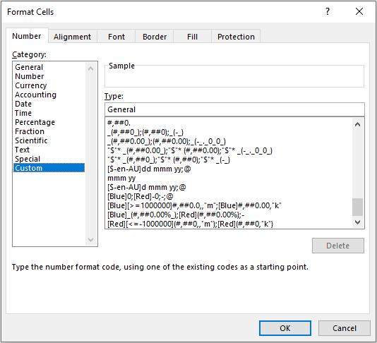
Given that one of the primary purposes of a spreadsheet is to present numerical data, it is important how numerical data is presented.  Cells may be individually formatted, using CTRL + 1 or ALT + O + E in all versions of Excel:

Formatting only changes the appearance, not the underlying value, of a cell. For example, if cells A1 and B1 had the number ‘1.4’ typed in but were formatted to zero decimal places, then if cell C1 = A1 + B1, I would truly have 1 + 1 = 3 (well, 1.4 + 1.4 = 2.8 anyway).

Excel has many built-in number formats that are fairly easy to understand, e.g. Currency, Date, Percentage. Selecting the ‘Custom’ category activates the ‘Type’ input box and allows between 200 and 250 custom number formats in a particular workbook, depending upon the language version of Excel that has been installed.

The ‘Type’ input box allows up to four aspects of formatting to be specified in a cell. These aspects are referred to as sections and are separated by a semi-colon (;). To ascertain what is contained in each section depends on the total number of sections used, viz.

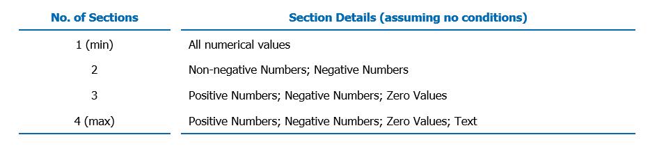
Notice only four options are available: what to do if positive, negative, zero or text.

There is an alternative syntax to the above four arguments:

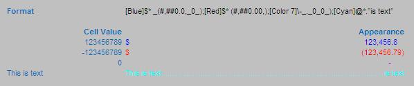
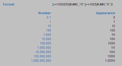
This may be demonstrated as follows:

The conditions are included in square brackets such that if the condition is true, the following formatting will be applied.

In this example, there are only three sections, so text will be formatted ‘generally’. The first section, [>=1000000]#,##0,,"M", will format all numbers greater than or equal to a million to the nearest million and add an “M” to the end of the number.

The second section will only be considered if the first condition is not true, so the order of the two ‘conditional formats’ needs to be thought through. Here, the second section, [>=1000]#,##0,"K", will format all numbers greater than or equal to a thousand (but necessarily less than a million) to the nearest thousand and add a “K” to the end of the number.

The third and final section, 0, will format all other numbers (every value less than 1,000) to the nearest integer without thousands separator(s).

This example is almost what we require; but it only allows three scenarios. We have many more.

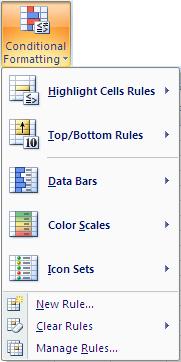
The trick here is to resort to conditional formatting. Located in the Styles group of the Home tab, the conditional formatting feature allows you to consider multiple conditions:

For instance, inspecting ‘Highlight Cells Rules’ is akin to many of the “Cell Value Is” functionalities of its predecessor, e.g. Greater Than, Less Than, Between, Equal To. I can use this to exploit a loophole in the restrictive number of conditions custom number formatting appears to allow. For example:

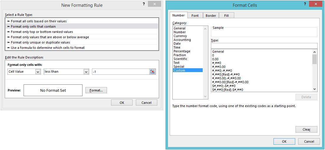
In this above illustration, I have selected conditional formatting to occur if the value in the cell is less than -1. Pressing the ‘Format…’ button then allows the user to select how the number formatting might appear.

Returning to my data:

Using both functionalities, the requirement is fairly straightforward. My suggested solution would be:

• Construct the underlying number formatting first. Personally, I would use custom number formatting so that all positive and negative numbers appeared as percentages, zero as a hyphen (“-“) and text as displayed above;
• Next, I would apply conditional formatting number formatting where the cell value is greater than one so that numbers greater than a million could be displayed to the nearest 0.1m, numbers less than a million but greater than or equal to 1,000 could be displayed to the nearest 0.00k and numbers lower than 1,000 (but necessarily greater than one) could be displayed as integers
• Finally, I would apply a second set of conditional formatting where the cell value is less than -1 as required.

I do not go through the required syntax here. My suggested solution can be found in the associated file. Since many, many conditional formats may be applied to one cell in Excel, you can soon apply significantly more than four formats to any cell(s) in Excel.

Next time I will move onto the next step where I create the chart.

That’s it for this week. Come back next week for more Charts and Dashboards tips.