Using OFFSET for Depreciation

Liam Bastick highlights some of the more useful functions for financial modelling / Excel spreadsheeting.  Liam explains how OFFSET can assist with change your perspective about modelling depreciation...

OFFSET reset

Last time I explained the OFFSET function: 

The arguments in square brackets (Height and Width) can be omitted from the formula – but they will prove to be useful in this article. 

As I explained last time, OFFSET(Reference,Rows,Columns) will select a reference Rows rows down (-Rows would be Rows rows up) and Columns columns to the right (-Columns would be Columns columns to the left) of the Reference.  For example, consider the following grid:

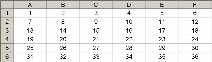
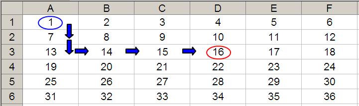
OFFSET(A1,2,3) would take us two rows down and three columns across to cell D3.  Therefore, OFFSET(A1,2,3) = 16, viz.

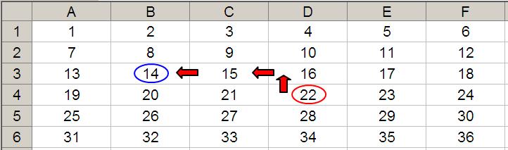
OFFSET(D4,-1,-2) would take us one row up and two columns to the left to cell B3.  Therefore, OFFSET(D4,-1,-2) = 14, viz.

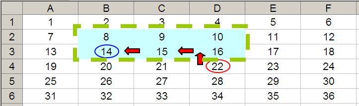
For Part 2 of this discussion, let me extend the formula to OFFSET(D4,-1,-2,-2,3). It would again take us to cell B3 but then we would select a range based on the Height and Width parameters.  The Height would be two rows going up the sheet, with row 14 as the base (i.e. rows 13 and 14), and the Width would be three columns going from left to right, with column B as the base (i.e. columns B, C and D).  

Hence OFFSET(D4,-1,-2,-2,3) would select the range B2:D3, viz.

Note that OFFSET(D4,-1,-2,-2,3) = #VALUE! since Excel cannot display a matrix in one cell, but it does recognise it.  However, if after typing in OFFSET(D4,-1,-2,-2,3) we press CTRL + SHIFT + ENTER, we turn the formula into an array formula: {OFFSET(D4,-1,-2,-2,3)} (do not type the braces in, they will appear automatically as part of the Excel syntax).  This gives a value of 8, which is the value in the top left hand corner of the matrix, but Excel is storing more than that.  This can be seen as follows:

• SUM(OFFSET(D4,-1,-2,-2,3)) = 72 (i.e. SUM(B2:D3))
• AVERAGE(OFFSET(D4,-1,-2,-2,3)) = 12 (i.e. AVERAGE(B2:D3)).

I am going to use these ideas to build on the scenario table example I demonstrated last time.  This time, I am going to consider a calculation many accountants have to perform regularly: depreciation of capital expenditure.

Example

Let’s imagine I have been charged with creating a depreciation schedule in an Excel spreadsheet with the following assumptions:

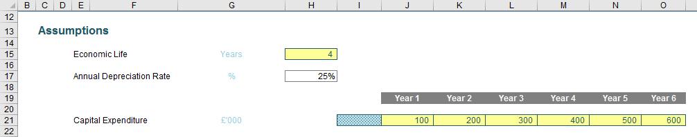
You can follow this example in the attached Excel file.  All cells in yellow are assumptions that may be changed. 

I wish to build a depreciation grid to calculate my total amortised cost as follows:

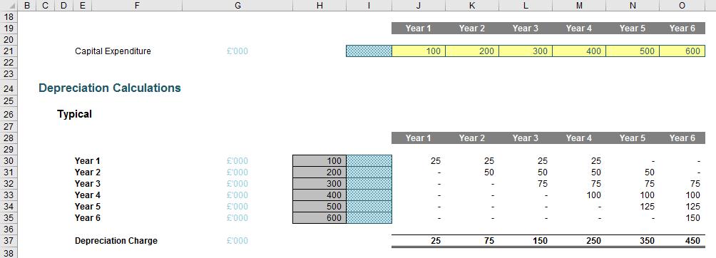
My first challenge is to link the assumptions in cells J21:O21 to the grey cells H30:H35, converting row assumptions into column data.  Converting from rows to columns (or vice versa) is known as transposing.  There are several ways you can do it, but only one way I truly recommend.

Method 1: Cut and Paste a Formula 

For the purposes of simplification, I am going to assume that we are looking to transpose data from going across a row to going down a column (the concepts are similar if columns are transposed into rows).

This method is very simple.  First, create a formula that links to the data to be transposed, say, in the row beneath:

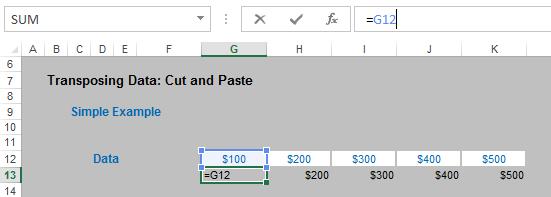
Second, once the formulae have all been created, cut and paste each formula individually into its appropriate position on the spreadsheet:

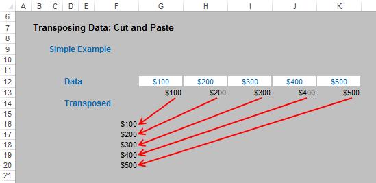
This is a very simple method, but certainly would be an ill-advised approach if you need to transpose 1,000 data points, for example.  

However, simplicity is often a highly-underrated attribute in modelling.  If you only have a few data items and you require the original inputs to remain (in our example, row 12, above), this method can often be deemed “simplest bestest”.

Method 2: Copy and Paste Special, Transpose

Another very simple approach is to copy and paste special as follows:

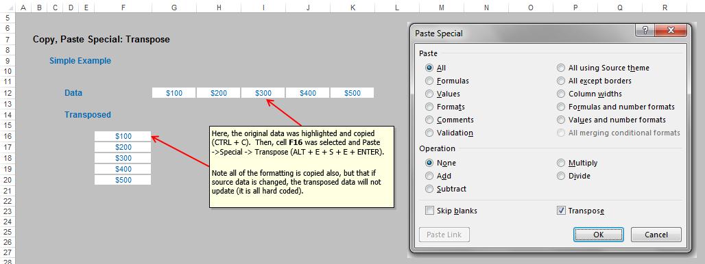
In this instance, simply highlight the data and copy the range in the usual way (e.g. CTRL + C).  Next, simply select the first cell (i.e. the top left hand corner) of the intended range and Paste Special, Transpose (ALT + E + S + E + ENTER).  As can be plainly seen from the illustration (above), the formatting as well as the content will be transposed.  

This is an ideal approach for copying and transposing data from one source to another where links are not required.  Aside from the inherited formatting, the main disadvantage here though is that depending upon the nature of the source data and how it is copied, updates in the original data will not flow through to the destination range. 

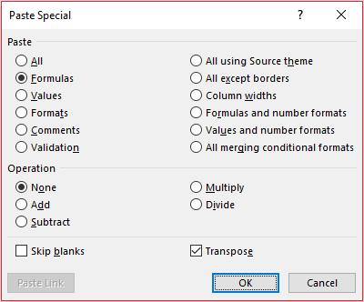
If the data needs to be linked to the source, then this approach is probably inappropriate.  However, if inherited formatting is all that is putting you off, make the appropriate adjustments to the ‘Paste Special’ dialog box before pressing ‘OK’ / ENTER, e.g. set the dialog box as follows to copy only the formulae before transposing:

Method 3: Using the TRANSPOSE Function 

On first glance, this looks like the ‘best’ method.  Once you discover there is a TRANSPOSE function, you think life is simple and your problems (well, you modelling problems anyway!) are over.  Unfortunately, this function is not without its limitations. 

Consider the following example:

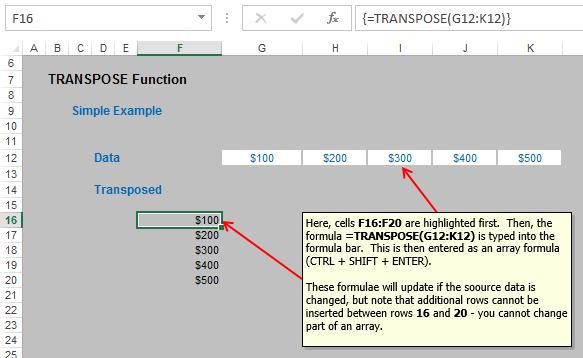
Here, the intention is to transpose the values in cells G12:K12 into the range F16:F20.  To do this, simply highlight cells F16:F20 and then type in the following formula: 

but rather than press ENTER, press CTRL + SHIFT + ENTER to enter the formula as an array formula.

This method is very simple, as long as you ensure that the destination range contains precisely the same number of cells in the column as there are cells in the source row.  If you change the source data, the outputs will update accordingly too. 

So what’s the problem? 

Array formulae can consume memory exponentially, which in turn can soon prevent Excel from calculating correctly, especially if you are working on a Windows 32-bit operating system, which is the platform most businesses employ. 

Further, if you wanted to insert additional rows between rows 16 and 20 (e.g. to extend the range), you will find that this is not possible:

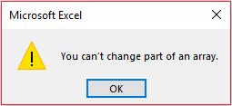
Only Chuck Norris can change part of an array, and unfortunately, he’s not available. 

Interestingly, if you insert columns between G and K in the illustration above, this is possible, but the array formulae will not act like other Excel calculations: cell references in the TRANSPOSE formulae will not update (so the references will always link to what is in cells G12:K12 in our example).  However, if you insert columns before column G, the formula will update.  This can be confusing.

Therefore, TRANSPOSE is useful where you wish to protect the destination range’s structure, but it can be seen as inflexible and inefficient, particularly with larger Excel files, slowing calculation times down unnecessarily.

Method 4: OFFSET Approach

Used with the ROWS function (which simply counts the number of rows in a specified range), transpositions may be performed quickly and effectively using OFFSET:

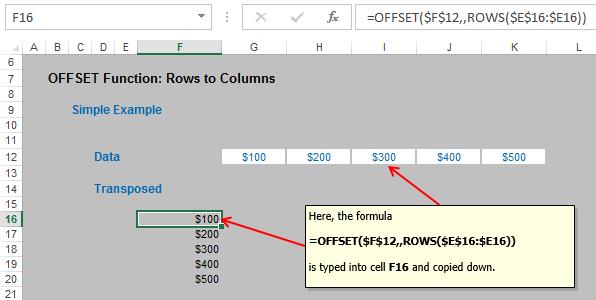
In this example, the following formula has been typed into cell F16: 

As the formula is copied down, the number increases in the columns argument of OFFSET, as the number of rows increases.  This is a neat trick for transposing without using array formulae, and can be seen as a good “general” solution, being quite flexible.  The disadvantages here are twofold:

• Often modellers make mistakes in the absolute and semi-absolute references required to make this formula calculate correctly.  This is easily overcome with practice; and
• The formula can look unnecessarily complex to the inexperienced or uninitiated.  There are many end users (and modellers for that matter) unfamiliar with the OFFSET function in particular. It may be worthwhile to educate them accordingly.

Returning to the Example

It is this last method I have employed in my depreciation example:

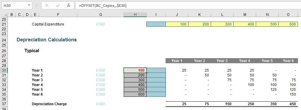
The formula in cell H30 (highlighted) is 

BC_Capex is cell I21.  The prefix “BC” in this range name stands for “Base Cell” and is used to acknowledge the fact that OFFSET is non-auditable, as explained last time.  This cell is styled speckled blue to emphasise that this cell must deliberately remain blank and not be deleted.  I use this “Empty Cell” style regularly in modelling. 

The reference $E30 points to the label “Year 1” which is actually the number 1 formatted to look like text.  This dispenses with the need to use the ROWS function explained earlier. 

Now that I have successfully transposed the assumptions, I can calculate the depreciation grid:

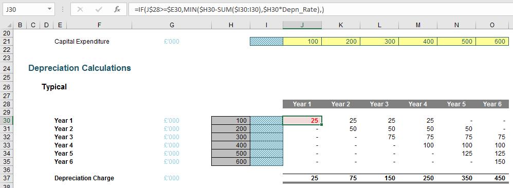
Assuming depreciation is to be calculated on a straight-line basis (i.e. the capital expenditure is apportioned equally across all periods it will provide economic benefit), the depreciation may be calculated across the grid using the formula in cell J30:

=IF(J$28>=$E30,MIN($H30-SUM($I30:I30),$H30*Depn_Rate),)

The IF statement checks that depreciation does not commence before the capital expenditure has occurred.  The MIN function takes a proportion of the capital expenditure but ensures that the cumulative total (“accumulated depreciation”) does not exceed the amount spent.

It is a simple method, recognised by many financial analysts and accountants.  The main problem with this method concerns how many calculations are required in the grid.  For example, if you built a 20-year monthly model, you would need 240 rows by 240 columns in the grid – a total of 57,600 calculations!

This is where OFFSET can come to the rescue… 

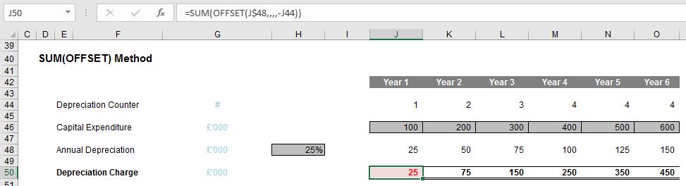
In this example, row 44 contains the formula =MIN(J42,Economic_Life) which restricts the period counter to not exceed the Economic_Life (here, four years).  With row 48 calculating each period’s representative depreciation, the total depreciation charge in row 50 becomes trivial.  For example, the formula in cell J50 is:

This formula simply refers to the corresponding periodic charge in row 48 and then sums a range of cells of width the negative value given in row 44.  This means that:

• In Period 1, depreciation is simply given by cell J48
• In Period 2, the depreciation is the sum of the first two charges in row 48 (namely, cells J48:K48)
• In Period 3, the depreciation is the sum of the first two charges in row 48 (namely, cells J48:L48)
• In Period 4, the depreciation is the sum of the first two charges in row 48 (namely, cells J48:M48)
• In Period 5, the depreciation is the sum of the first two charges in row 48 (namely, cells K48:N48).  Note that the first period is now excluded (the width is -4) as the first period’s capital expenditure is now fully depreciated.

A simple comparison of the two approaches to depreciation will determine that the two methods give the same result.  The OFFSET approach may not be as transparent upon first glance, but it does reduce the number of formulae required. 

When I model depreciation in reality, I usually model the first asset class both ways so that end users may see they give the same result.  After that, I adopt the OFFSET approach exclusively as end users now “trust” this less familiar approach. 

I recommend if you are not familiar with OFFSET you should do the same.  Play with the function for a while until you trusty it and realise how useful it can be in your spreadsheets going forward.