Spreadsheet Skills: Unique Rank

How do your spreadsheet skills RANK? Do you know how to order numerical data when there are duplicates or blanks? It’s easier than you think. By Liam Bastick, Managing Director (and Excel MVP) with SumProduct Pty Ltd.

Query

I have a list of numerical data that I need to rank from smallest to largest. I am aware of the RANK function in Excel but it does not seem to cope with duplicate values. Can you advise?

Advice

For this query, let me construct an example (which is replicated in the attached Excel file):

Here, there are 10 items, with several duplicates and one blank value. That should be plenty to make this example sufficiently awkward!

To order this data, we can use the RANK function:

where:

• number is the value to be ranked.  It should be noted that the RANK value only works with numbers (this is why the last rank in the example below is #N/A – the value is a blank cell; text will create #VALUE! errors);
• list is the range of numbers that are to be ranked.  This should be a column or row vector (i.e. the range consists of only one row or only one column); and
• ranking_order is an optional argument.  This is why it is in square brackets (do not put the value in square brackets!).  If the value is 0 or omitted, the ranking is descending (largest first), whereas if it is 1, the ranking is ascending (smallest first).

The following example employs a simple RANK formula:

This example clearly demonstrates the problems:

• As explained above, non-numeric values (e.g. cell G22) create prima facie errors in the results; and
• Duplicate values (e.g. rows 20 and 21) give the same ranking.  Do not be put off by number formatting: the value in cell G14 is actually 7.3 in our example, not 7 similar to the values in cells G20 and G21.

We need to create a formula that removes both of these obstacles.  The following is one such calculation when ranking is to be performed in ascending order:

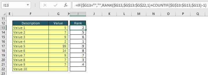
The formula in the first cell in our example is:

The IF condition checks for blank cells and thus avoids #N/A errors. If a more comprehensive error check is required, you may use 

instead.

The COUNTIF($G$13:$G13,$G13)-1 argument uses the COUNTIF(List,Criterion) function, where it counts the number of occurrences of the Criterion (value) in the List (range).  In this instance, the first occurrence adds zero to the ranking, the second a value of one and so on.  Note that List in this example expands as you move down the range.  This deals with duplicates adding a “tie-breaker”.  The logic works the same for both ascending and descending ranking.

Word to the Wise

It does not take much imagination to make this example more sophisticated and this is demonstrated in the attached Excel file.  Data validation (see >Data Validation) may be used to create a switch between an ascending and a descending sort and INDEX MATCH (see >Index Match) may be employed to summarise the re-sorted data.

If you have a query for the Spreadsheet Skills section, please feel free to drop Liam a line at liam.bastick@sumproduct.com