
Summing a Dynamic Range
Especially at this time of year, as accountants, we often want to sum data for a period of time, e.g. sales for the last quarter, year to date costs and rolling budgets / forecasts. When we create these calculations “statically”, i.e. the range is specified explicitly.
For example, we might have something like the following example:
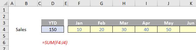
Here, we have created a static formula for the year to date sales using the calculation
=SUM(F4:J4)
Next month, we would have to update this to
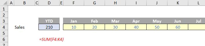
We can’t simply sum the range in case other users populate row 4 with forecast estimates, etc. There is an alternative, and I thought I would go up to date and use Excel 365’s XLOOKUP function.
As a reminder, XLOOKUP has the following syntax:
XLOOKUP(lookup_value, lookup_vector, results_array, [if_not_found], [match_mode], [search_mode])
This function seeks out a lookup_value in the lookup_vector and returns the corresponding value in the results_array. It may seem complex, but most of the time you will only require the first three arguments:
- lookup_value: this is required and defines what value you want to look up
- lookup_vector: this reference is required and is the row or column of data you are referencing to look up lookup_value
- results_array: this is where the corresponding item is you wish to return and is also required (even if it is the same as lookup_vector). This does not have to be a vector (i.e. one row or one column of cells): it may be an array (with at least two rows and at least two columns of cells). The only stipulation is that the number of rows / columns must equal the number of rows / columns in the column / row vector – but more on that later.
For the record, the remaining arguments are:
- if_not_found: this optional argument allows you to replace the usual return of #N/A with something more informative like an alternative formula, text or a value
- match_mode: this argument is optional. There are four choices:
- 0: exact match (default)
- -1: exact match or else the largest value less than or equal to lookup_value
- 1: exact match or else smallest value greater than or equal to lookup_value
- 2: wildcard match. You should use the special character ? to match any character and * to match any run of characters.
What’s impressive, though, is that for certain selections of the final argument (search_mode), you don’t need to put your data in alphanumerical order! As far as I am aware, this is a first for Excel
- search_mode: this argument is also optional. There are again four choices:
- 1: search first to last (default)
- -1: search last to first
- 2: what is known as a binary search, first to last (requires lookup_vector to be sorted). Just so you know, a binary search is a search algorithm that finds the position of a target value within a sorted array. A binary search compares the target value to the middle element of the array. If they are not equal, the half in which the target cannot lie is eliminated and the search continues on the remaining half, again taking the middle element to compare to the target value, and repeating this until the target value is found
- -2: another binary search, this time last to first (and again, this requires lookup_vector to be sorted).
Let’s have a look at XLOOKUP versus everyone’s favourite function (except me!), VLOOKUP:
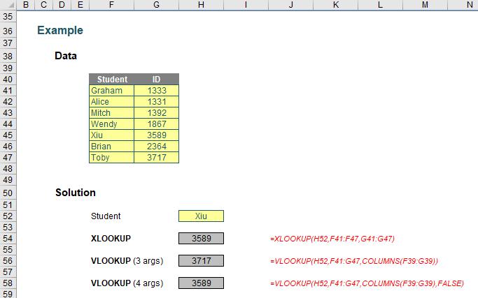
You can clearly see the XLOOKUP function is shorter:
=XLOOKUP(H52,F41:F47,G41:G47)
Only the first three arguments are needed, whereas VLOOKUP requires both a fourth argument, and, for full flexibility, the COLUMNS function as well. XLOOKUP will automatically update if rows / columns are inserted or deleted. It’s just simpler.
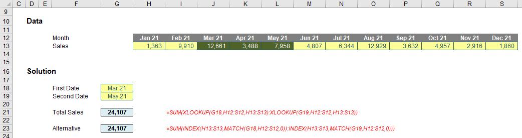
We can use this to specify the start and end of our sum range as follows. Consider the following example:
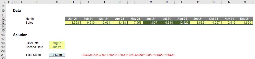
The formula is “simply”
=SUM(XLOOKUP(G18,H12:S12,H13:S13):XLOOKUP(G19,H12:S12,H13:S13))
This is just two XLOOKUP functions joined together within a SUM function, specifying the start and end of the range. Indeed, if the First Date is after the Second Date it will still work. The SUM function is not precious and will work in “reverse order” too.
The dates may be varied and the summation updates both automatically and correctly, viz.
Simple!
Word to the wise
For those who are getting upset at this point because they don’t have access to Excel 365 and / or the XLOOKUP function, do not despair. The old faithful INDEX(MATCH) combo still works. It’s just clunkier:
=SUM(INDEX(H13:S13,MATCH(G18,H12:S12,0)):INDEX(H13:S13,MATCH(G19,H12:S12,0)))
Lovely! Until next time…