Running in a Field

We look at how to create running totals and similar devices in a Table – it’s trickier than it sounds. By Liam Bastick, director (and Excel MVP) with SumProduct Pty Ltd.

Query

HELP!  I am trying to add a unique counter to a table of data in an Excel Table and it’s not working correctly.  What am I doing wrong?

Advice

First introduced in Excel 2007, I have extolled the virtues of Excel Tables before (please see the Tables Thought article for past details).  As a gentle reminder though…

Refresh on Tables

Creating a Table in Excel 2007 and later versions is straightforward, and simply requires the user to select the data to be used in the Table.  You do not even need to select the whole range: Excel will prompt for the whole Table even if only one cell is selected (PivotTable creation works similarly).

Next, from the Ribbon, in the ‘Styles’ group of the ‘Home’ tab, click on the button that says ‘Format as Table’:

Format as Table

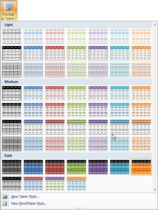
After clicking this button, Excel shows a new user interface element called a gallery, with a number of formatting choices for your Table, as displayed above.  New styles may be created by selecting ‘New Table Style…’ if required.

After one of the formats has been chosen, Excel will prompt the user regarding which cells are to be converted to a Table:

Create Table dialog box

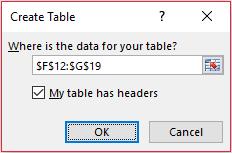
If the Table contains a heading row, ensure that the ‘My table has headers’ checkbox is checked.  Click ‘OK’ to convert the range to a Table.  The keyboard shortcut CTRL + T will have the same effect without allowing you to choose the formatting.

Tables have various useful functionalities, one such being the filtering which was done in lists in Excel 2003 and earlier versions.  For example, provided the Table has a header row, it will always have in-built filter and sorting, which can be readily accessed from this top row.

A Table will automatically resize to accommodate additional rows and / or columns, provided that data is entered in a cell immediately after the last column or row.  It is this feature that is particularly useful when dealing with our lists problem.

So What’s the Problem?

If a formula is entered in the first cell for a given field, it will propagate throughout the column, e.g.

Bad Counter Example

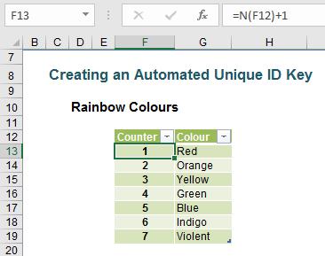
This example adds one to the value in the cell above; the N() function simply treats text as zero rather than generate an #VALUE! error.  It seems to look fine.  The problem occurs when rows are inserted into the Table:

Bad Counter Example Demonstrated

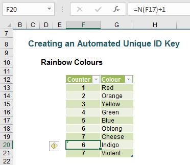
Do you see what has happened?  The formulae after the insertion point continue as if the added rows never occurred.  It is very easy to miss this in practice and this can cause errors in reports etc.  It needs to be avoided.

There are various solutions, although personally I think alternatives based our old favourite function, INDEX(), are some of the most flexible:

Counter Issue Solved with INDEX

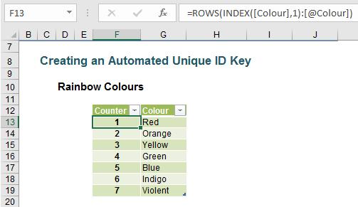
Ah yes, that’s erm very obvious.  Perhaps I need to explain slightly:

• The ROWS() function simply counts the number of rows in a range.  In this instance the range is denoted by INDEX([Colour],1):[@Colour]).  This syntax may vary slightly depending upon whether you are using Excel 2007 or Excel 2010 and later versions.
• In Excel 2010 and later, [Colour] denotes the range G13:G19 in our example (highlighting this range will cause [Colour] to appear).
• INDEX([Colour],1) means take the first cell reference in the range.  This is cell G13 in our example and it essentially anchors this cell, i.e. it is the equivalent of $G$13.
• [@Colour] in Excel 2010 and later is generated whenever a formula refers to a cell in the field [Colour] in the same row as the formula, so in cell F13, the reference [@Colour] is referring to the variable in cell G13.
• In essence, the Table formula is calculating =ROWS($G$13:G13) – but in a way an Excel Table can understand.
• In Excel 2007, Table formula syntax was different:

Counter Issue Solved with INDEX (Excel 2007 Syntax)

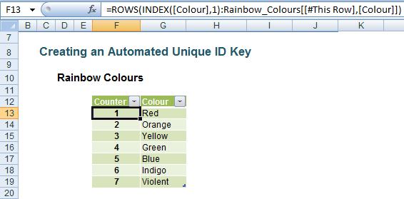
Rainbow_Colours refers to the name of the Table in this example.

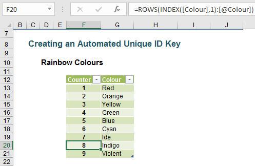
This formula may appear to be more cumbersome and convoluted but it does do the trick as adding rows will attest:

Counter Issue with Rows Added

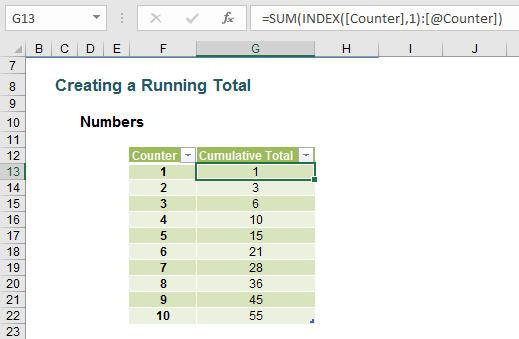
It doesn’t take much to extend this idea.  Counters are very important in order to automatically generate row identifiers, but running totals can be useful too (simply swap the ROWS() function for the SUM() function):

Running Totals Example

If you only want to sum the visible rows, that’s easy too:

Summing Visible Amounts Only Example

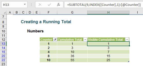
That’s right, I am back to the SUBTOTAL(9,) function again (please see the SUBTOTAL Function and Functionality Thought article for further details).  It’s the same idea over and over again though.

As usual, the attached Excel file shows you the above examples, working in all versions of Excel from Excel 2007.

Word to the Wise

Don’t type the formulae in from this article: actually create the Tables and generate the syntax by clicking on the cell or cells.  By doing this, you will better understand how Tables work and it will make the confusing nomenclature a little clearer (hopefully!).

If you want to read more on cell formatting we have an article on Styles, otherwise please feel free to drop Liam a line at liam.bastick@sumproduct.com