
Revising Forecasts
Liam Bastick, director (and Excel MVP) with SumProduct Pty Ltd, takes a look at how to revise forecasts as timing(s) move.
All Change Please
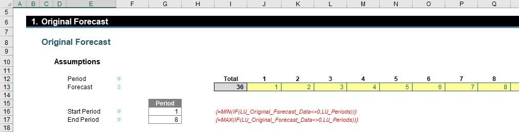
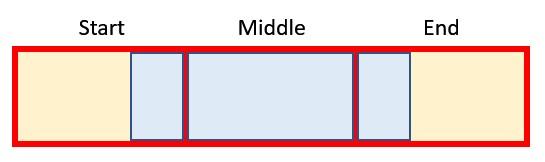
Imagine you had just finalised the budget for a project and (say) it started in Period 3 and ended in Period 8 as pictured:
Suddenly, your boss told you the amounts needed to be reallocated on a “similar basis” but for Periods 4 to 15. That’s fairly straightforward, as this duration is double the original project length, so you would just attribute half of each period’s amount to the new periods, viz.

But what about a general solution? How would you cope with project advancements or delays and changes in duration at the same time? It sounds pretty horrible, but truth be told, finance staff face these types of challenge day-in, day-out.
Assuming no inflationary factors to consider (e.g. time value of money), the problem boils down to pro-rating the original numbers across the new number of periods. The revised start and end dates tell you when the calculations begin, but in essence it is the number of periods in the revised forecast that drives the calculations.
You can follow our explanation in the attached Excel file.
Sorry for the algebra, but sometimes that’s what’s needed in a financial model! Let’s assume our original forecast has x periods going from start period t1 to end period tx, and the revised forecast has y periods going from revised start period r1 to revised end period ry.

In this illustration, r1 occurs after t1, but this does not have to be true necessarily.
Regardless of start and finish dates (which simply governs when the calculations are made), there are basically three scenarios:
- x > y, i.e. the revised forecast duration is shorter than the original one
- x < y, i.e. the revised forecast duration is longer than the original one
- x = y, i.e. the durations of both forecast periods are equal (this effectively simply moves the forecast period).
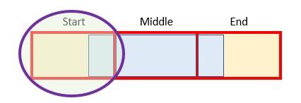
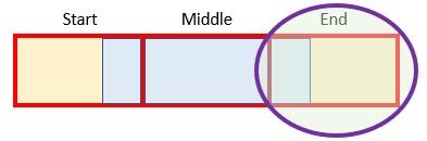
Let’s focus on the first scenario for a moment as it brings into focus how we could go about calculating the revised forecast. If the original duration were longer, then the revised forecast will consider the effects of more than one original period in each period, e.g.

In this graphic, the red boxes / yellow shading represent original periods and the blue boxes / borders denote a revised period. If x > y, then the blue box must straddle at least two red boxes. It could be more though, which is what is depicted here, where we have:
- a start period, where this is the proportion of the earliest original period considered
- middle [or full] period(s), which (when x > y) are original periods that must be fully included. There could be more than one. If x < y, middle (full) period is not defined
- an end period, which is the proportion of the final original period considered.
Sounds confusing? Let’s explain with an example:

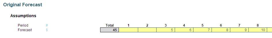
In the original forecasts, the cashflows of $1 to $8 (big spenders here!) were allocated across the first eight periods for a total of a rather exorbitant $36. However, the revised forecast wanted the same profile over just periods 4 to 6 (three periods). That is, the start date t1 is period 1, x is 8 and the final period tx (t8) is period 8.
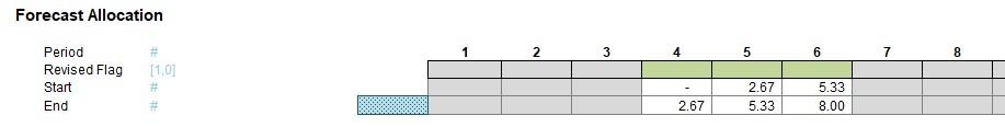
The start and end dates (r1 and r3, periods 4 and 6 respectively) for the revised forecast just denote when the forecast starts and stops. The key information is that there are only 3 (y) periods. This means that each period in the revised forecast includes 8/3 (known as the Period Factor in the attached Excel file) which equals two and two-thirds (2.67) periods of the old forecast data viz.
- Revised Period 4 = Old Period 1 + Old Period 2 + 2/3 of Old Period 3 = 1 + 2 + (2x3)/3 = 5
- Revised Period 5 = 1/3 of Old Period 3 + Old Period 4 + Old Period 5 + 1/3 of Old Period 6 = (1x3)/3 + 4 + 5 + (1x6)/3 = 12
- Revised Period 6 = 2/3 of Old Period 6 + Old Period 7 + Old Period 8 = (2x6)/3 + 7 + 8 = 19.
Our attached Excel file identifies which original periods are used in each revised period,
what the start, middle / full and end periods are,
And what proportions to use of each:
These then cross-multiply the original forecast numbers for the appropriate periods using the SUMIF and SUMIFS functions to get the values explained above.
When the revised forecast period is longer than the original one, the problem is slightly simpler as there are no middle / full periods (i.e. no period of original data is ever in just one revised period). Otherwise, the logic remains the same.
For those who are interested or are insomniacs, the detail is discussed below…
Devil’s in the Detail
Let’s use the attached Excel file to talk through the formulae we used.
The first section captures the original forecast (inputs) in cells J13:Q13 and automatically computes the start and end period using the array formulae for MIN(IF) and MAX(IF) (cells G16 and G17 respectively). These must be entered using CTRL + SHIFT + ENTER as IF will not work across a range (an array) of cells otherwise.
The next section is the Revised Forecast assumptions:
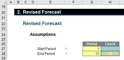
This collects the required start and end periods in cells G27 and G28, together with an error check in cell H28 to ensure that the end period is not before the start period.
The first part of the next section simply collates all of the date to be used:
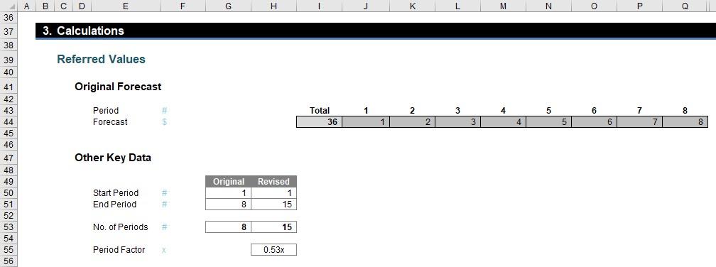
The key calculation here is the Period Factor (cell H55) which divides the original forecast duration by the revised forecast duration. This represents the number of original periods in each revised period and this is pivotal to all of the calculations.
The next part of this section works out how the original periods are reallocated to the revised periods:
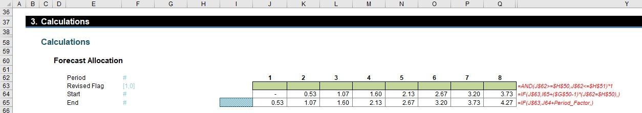
The Revised Flag (row 63) use the formula
=AND(J$62>=$H$50,J$62<=$H$51)*1
to check that the period counters in row 62 are greater than or equal to the revised start period (H50) and less than or equal to the revised end period (H51). The value is 1 if these assumptions are true and zero (0) otherwise.
The formula for the Start (row 64),
=IF(J$63,I65+($G$50-1)*(J$62=$H$50),)
is a simple formula that takes the previous period’s closing balance (as long as the flag is active) but also accounts for the fact that the original forecast may not have occurred in Period 1 (i.e. it sets the first period t1 of the original forecast period).
The final formula for the End (row 65),
=IF(J$63,J64+Period_Factor,)
simply adds the Period Factor to the Start period as long as the flag is active. This gives us ultimately the beginning and the end of the blue section in our graphic from before:
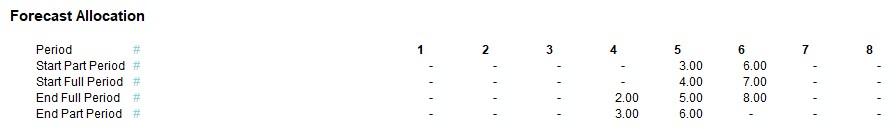
The next section starts working out which original periods need to be considered for the start, middle (full) and end:
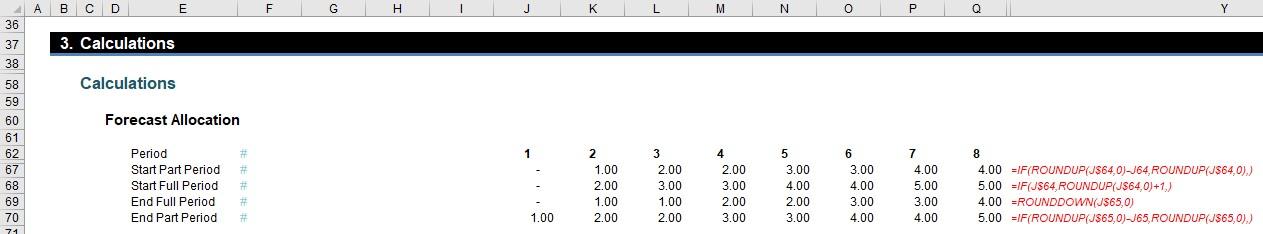
The Start Part Period uses the formula
=IF(ROUNDUP(J$64,0)-J64,ROUNDUP(J$64,0),)
Essentially, if Start (row 64) is an integer it uses that period number otherwise it uses the next period (ROUNDUP(z,0) rounds z up to zero decimal places, i.e. the next whole number).
Rows 68 and 69 establish the beginning and the end of the middle (full) period – sort of. Row 69, the calculation for the Start Part Period,
=IF(J$64,ROUNDUP(J$64,0)+1,)
adds one to the Start Part Period (row 67) (as long this is not zero) to avoid any double count. Row 69’s formula for the End Full Period,
=ROUNDDOWN(J$65,0)
takes the “beginning of the end”, that is, up to but not including the End period. Therefore, the way these two dates are calculated it is possible that the Start Full Period could be a period prior to the End Full Period. That is actually pictured in our example (above) and is acceptable – it simply means there is no full / middle period in that instance.
The final formula here (row 70) for End Part Period,
=IF(ROUNDUP(J$65,0)-J65,ROUNDUP(J$65,0),)
uses the same logic as per the Start Part Period. This means we now have the relevant original periods identified!
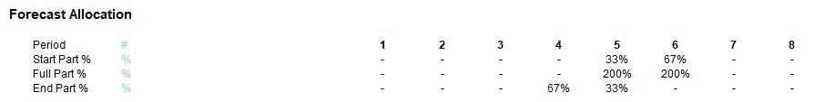
Next, we need to know what percentages should be used for Start and End Part Periods.
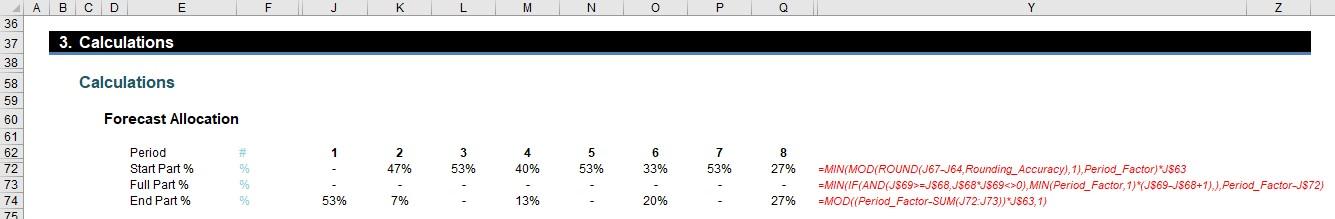
The Full Part % is also calculated as it ensures the End Part % is not overstated.
The formula in row 72 for the Start Part %,
=MIN(MOD(ROUND(J67-J64,Rounding_Accuracy),1),Period_Factor)*J$63
looks horrible but isn’t as bad as it seems (honest)! J67-J64 calculates the proportion Start Part Period less Start (i.e. this formula computes the proportion of the first red box that is blue).
ROUND is used to prevent rounding errors and MOD is incorporated to ensure this proportion is less than 100% (I’ve discussed MOD in a previous article or two).
The second formula is not pleasant either. The Full Part % (row 73) is given by:
=MIN(IF(AND(J$69>=J$68,J$68*J$69<>0),MIN(Period_Factor,1)*(J$69-J$68+1),),Period_Factor-J$72)
Erm, lovely… Again, once you get your head wrapped around it, it’s not so bad. The two IF conditions required (inside the AND expression) check that the periods are not zero and that the end is not before the beginning (as discussed above). If this test is passed, it takes the MIN(Period_Factor,1) (you cannot count more than the forecast amount in an original period) and multiplies this by the number of full original periods in the revised period. This is then restricted so that the sum of the Start Part % and the Full Part % cannot exceed the Period Factor. This number is calculated only to keep the End Part % honest. Talking of which…
The End Part % (row 74),
=MOD((Period_Factor-SUM(J72:J73))*J$63,1)
just mops up the rest of the Period Factor where the flag is active. This is equal to the section highlighted:
This concludes the percentages needed. We now have identified which periods are the Start Middle and End and what proportions we require for the Start and End. “All” we have to do is multiply it out:
I say “all” because we’ve left the best to last…
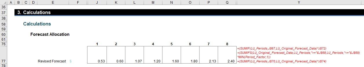
=(SUMIF(LU_Periods,J$67,LU_Original_Forecast_Data)*J$72)
+(SUMIFS(LU_Original_Forecast_Data,LU_Periods,">="&J$68,LU_Periods,"<="&J$69)*MIN(Period_Factor,1))
+(SUMIF(LU_Periods,J$70,LU_Original_Forecast_Data)*J$74)
Again, it’s really not that bad! There’s three calculations here = one each for the start, middle and end. The first one:
=SUMIF(LU_Periods,J$67,LU_Original_Forecast_Data)*J$72
locates the original period to be used for Start and multiplies it by the appropriate proportion (SUMIF only sums the range LU_Original_Forecast_Data where the counter in LU_Periods is equal to the value in cell J67, i.e. the correct original period to be used).
The last formula,
=SUMIF(LU_Periods,J$70,LU_Original_Forecast_Data)*J$74
performs a similar operation for the End period. This just leaves:
=SUMIFS(LU_Original_Forecast_Data,LU_Periods,">="&J$68,LU_Periods,"<="&J$69)*MIN(Period_Factor,1)
SUMIFS is used here as we need to sum based on two conditions, not one (that the full periods meet the conditions for the Start and End Full Periods). Here, you can clearly see if the End Full Period precedes the Start Full Period, no amounts will be summed. The factor MIN(Period_Factor,1) is required when the number of revised periods is greater than the original number of forecast periods (so only the correct proportion) is used and to ensure the amount in a full period is never multiplied by a factor greater than 1 also.
These three added together give us our total:

Word to the Wise
Anyway, apologies for this article being a little heavier than usual, but this is a common problem when revising forecasts in Excel. The solution may be a little involved, but I hope you will agree you can always “steal” my template and figure out the formulae at your leisure. This is the curse of modelling sometimes – not always is every essential calculation simple!
If you have a query for the Thought section, please feel free to drop Liam a line at liam.bastick@sumproduct.com or visit the SumProduct website.