Not Just Mary Can Have a Little LAMBDA / Excel Hits 500

It’s busy times in the land of Excel 365 – if you want to live on the cutting edge.  Microsoft has just announced the release of no less than seven new LAMBDA-associated functions (including a landmark 500^th one – someone please bake Excel a cake) for the Beta variant, whilst also moving the recently released LAMBDA function a step closer to becoming Generally Available.

It’s a lot to take in.  Where do we start?  Perhaps let’s begin with revisiting LAMBDA itself.

LAMBDA Moves to Excel 365 Current Channel Preview

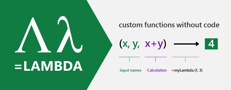
For those who have been hiding under a rock, let me start by saying LAMBDA rocks (if this continues, this will be a very short article – Ed.).  Simply put, LAMBDA allows you to define your own custom functions using Excel’s formula language.  It’s User Defined Functions without a PhD in VBA or JavaScript.  Now moved to the Office 365 Current Channel Preview from Beta, LAMBDA allows you to define a custom function in Excel’s very own formula language.  Moreover, one function can call another (including itself), so there is no limit to the power you can deploy with a single function call. 

As a reminder, the syntax of LAMBDA perhaps remains not the most informative:

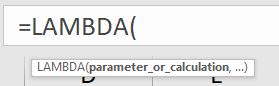
That’s, er, great.  Perhaps a run-through might be best.

There are three key pieces of =LAMBDA to understand:

1.      LAMBDA function components

2.      Naming a lambda

3.      Calling a lambda function.

1. LAMBDA function components

Let’s take a simple example.  Consider the following formula:

This is a very exciting formula, where we have x as the argument, which you may pass in when calling the LAMBDA, and x+1 is the logic / operation to be performed.

For example, if you were to call this lambda function and define x as equal to five (5), then Excel would calculate

Except it wouldn’t.  If you tried this you would get #CALC!  Oops.  That’s because it’s not quite as simple as that.  You need to name your little LAMBDA.

2. Naming a LAMBDA

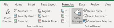
To give your LAMBDA a name so it can be re-used, you have to use the Name Manager (CTRL + F3 / go to the Ribbon and then go to Formulas -> Name Manager):

Once you open the ‘Name Manager’ you will see the following dialog:

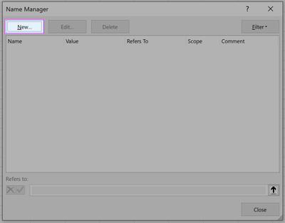
You then click on ‘New’ and fill out the related fields, viz.

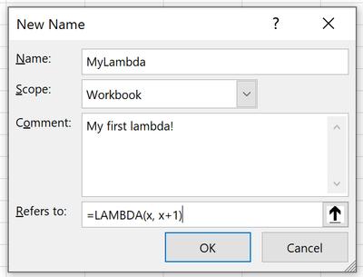
To be clear:

• Name: the name of your function (this is where you name it!)
• Comment: a description and associated ToolTip, which will be shown when calling your function
• Refers to: your lambda function definition (this is where you put your formula – NOT in the Excel worksheet!).

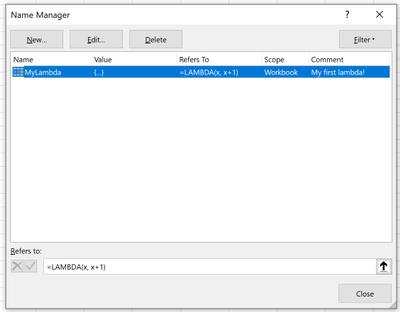
Once completed, you may press ‘OK’ to store your lambda and you should see the definition returned in the resultant window.

3. Calling LAMBDA

Now that you have done this, your first new lambda function may be called in just the same way as every other Excel function is cited, e.g.

which would equal six (6) and not #CALC! as before.

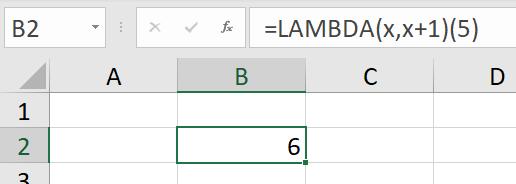
You DON’T have to do it this way though if you don’t want to.  You may call a lambda without naming it.  If we hadn’t named this marvellous calculation, and simply authored it in the grid as we had first attempted, we could call it by simply typing:

The sky’s the limit.  You are not restricted to just numbers and text.  You can also use:

• Dynamic arrays: rather than passing a single value into a function, you can pass an array of values, and functions can also return arrays of values
• Data Types: the value stored in a cell is no longer just a string or a number.  A single cell can contain a rich Data Type, with a large set of properties, as discussed previously.

Functions can take data types and arrays as arguments, and they can also return results as data types and arrays.  The same is now true with the lambdas you build.

Indeed, formulaic recursion is possible too, such as creating a Triangle number

using the lambda formula

Now, yes, I know you can use the calculation

but nobody likes a smart alec!  You get the point.

To celebrate LAMBDA moving to Current Channel Preview, Microsoft has also added support for optional parameters.  To make use of these new take-them-or-leave-them arguments, all you need to do is wrap the optional name in square brackets, “[]”, e.g.

(In case you have no idea what ISOMITTED does (I am sure you can guess!), don’t worry, it’s one of the new functions divulged below…)

Simply put, this lambda will return the value of arg1 if arg2 is omitted; otherwise, it will return the value of arg2.  I’d like to have called this lambda function Jason as it sort of checks if his args are naught, but sadly it’s not Friday 13^th…

The lambda function is available to members of the Current Channel Preview program running Windows and Mac builds of Excel, but is only available to a random 50% of users as at the time of writing.  Microsoft has stated that they will increase this “flight”, pending no bugs or other issues.

Introducing the New LAMBDA Helper Functions

LAMBDA now enhances Excel’s formula language, with its ability to be treated as an accepted value type with the introduction of these new functions.  This is an important concept, which has existed across many programming languages, and is tantamount to the concept of lambda functions in general, never mind just in Excel.

Recently, Excel has introduced new types of values.  This has included Data Types (Wolfram, Geography, Stocks, Power BI and Power Query can create Data Types) and dynamic arrays.  Lambdas continue these enhancements by allowing Excel to understand functions as a value.  This was enabled by the introduction of LAMBDA, but it requires support, which is what these seven new functions bring.

This means that previous Excel tasks which previously seemed practically impossible, may now be achieved by writing a LAMBDA and passing it as a value into another function.

Bring on the newbies…

BYCOL

BYCOL is not a region of the Philippines, but rather a function that takes an array or range and calls a lambda, with all the data grouped by each row or column and then returns an array of single values.  

Its syntax is as follows:

It has the following arguments:

• array: this is required, and represents an array to be separated by column
• lambda: an optional argument, this is a LAMBDA that takes a column as a single parameter and calculates just one result.

As an example, my co-author Chris and I have decided to make small talk and discuss the weather – in particular, whether we use Celsius or Fahrenheit as our temperature scale.  Chris uses Fahrenheit because he is based in the United States (more on this fact later) and I use Celsius because I am right.

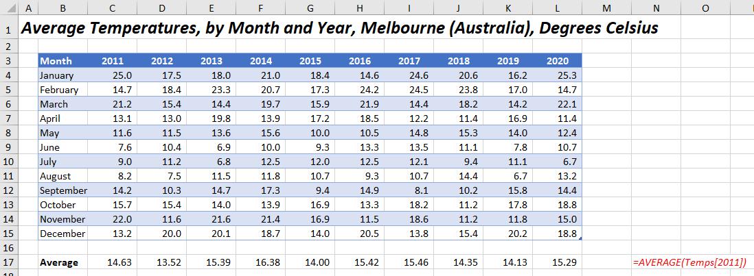
I have made up some average monthly temperatures for Melbourne (Australia), not that it matters given we are all in Lockdown:

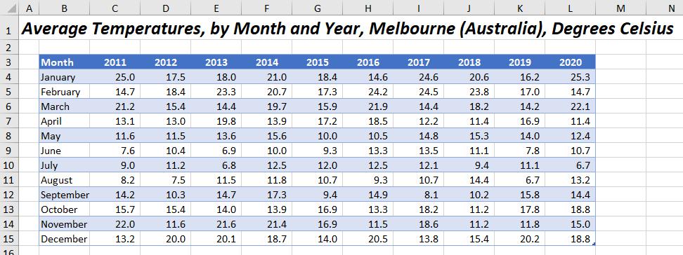
I have called this Excel Table Temps, but it is a permanent name…

For the years 2011 to 2020 inclusive, I want to provide a detailed monthly breakdown of temperatures where the average temperature for the year was above 15 degrees Celsius.  At this point, you would normally calculate the average temperature for each column using a formula such as

for column C of this example spreadsheet.

This would be a “helper row”, e.g.

But I am not going to do it that way. Instead, let’s use BYCOL.  First of all, let’s see how it works.  Consider the calculation

Note I have used Temps as my array, which is cells B4:L15, i.e. it omits the header row of the table (cells B3:L3).  I have to ignore the headers because the years would be included in the column totals being numbers – a classic gotcha!

This would produce the following result:

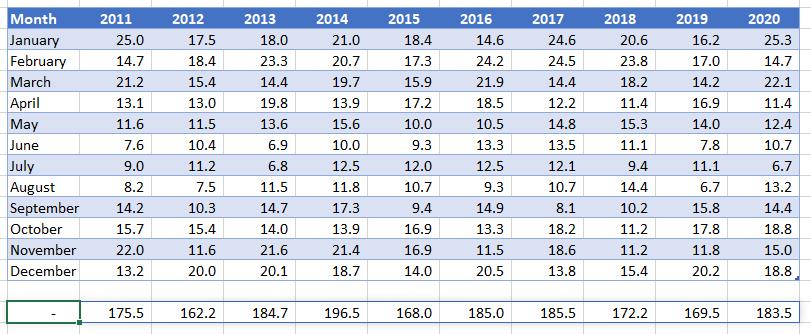
BYCOL produces a row vector, summing up each column of the table Temps, excluding the header row.  The formula spills, using dynamic array logic and matches the width of the underlying array (i.e. the Table Temps).  It only produces one row of data, as we have created a summation (just one value to report for each column).

Now, let’s consider the following formula:

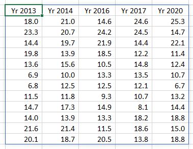
Here, BYCOL produces a row of TRUE or FALSE values, depending upon whether the average for each column exceeds 15 degrees Celsius.  The dynamic array function FILTER, one of the recently introduced dynamic array functions then filters each column in Temps based upon whether the corresponding LAMBDA equates to TRUE or FALSE, viz.

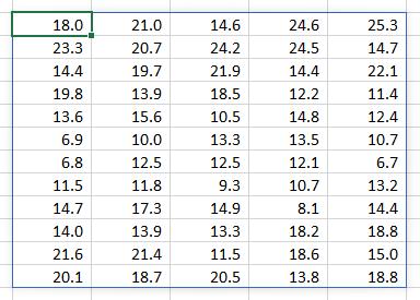
This returns the columnar data for the years 2013, 2014, 2016, 2017 and 2020 respectively – not that you would know from the above numerical dataset.  I really wanted the headings, but having numerical values in the Table header did not help my cause (it would have caused my averages to calculate incorrectly).  It is usually not a good idea to have numerical values in Table headers, and perhaps now you can understand why.

If I modify the Table’s headers as follows, I can now use the entire Table:

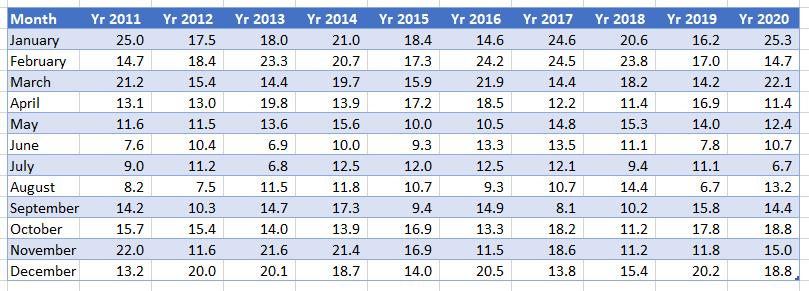
The formula may be modified to

which will produce a more informative spilled array:

BYROW

BYROW works very similarly to BYCOL (it is analogous to the relationship between HLOOKUP and VLOOKUP).  This function applies a LAMBDA to each row and returns an array of the results.  Its syntax is as follows:

It has the following arguments:

• array: this is required, and represents an array to be separated by row
• lambda: an optional argument, this is a LAMBDA that takes a column as a single parameter and calculates just one result.

Let’s return to my above example:

BYROW effectively produces a column vector, summing up each row of the table Temps.

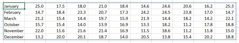
If I want the year-on-year comparisons for each month where the average temperature is above 15 degrees Celsius, I can again avoid using a “helper column” and instead use the formula

This time, I can ignore the header row.  This will return the array

Once you get the hang of these LAMBDA helper functions, you will begin to wonder how you ever managed without them.

ISOMITTED

This new function checks whether the value is missing, and returns either TRUE (value is missing) or FALSE (value is not missing) accordingly.  The syntax is simple:

where:

• argument is a required parameter, and is the value you want to test, which may be based upon a LAMBDA.

The example

was provided earlier, where this lambda will return the value of arg1 if arg2 is omitted; otherwise, it will return the value of arg2. 

MAKEARRAY

MAKEARRAY returns a calculated array of a specified row and column size, by applying a LAMBDA function.  This function is useful for situations where you wish to combine or transform arrays, as well as being useful for generating data.  The syntax is as follows:

It has the following arguments:

• rows: this argument is required and represents the number of rows in the array (which must be greater than zero)
• columns: this argument is also required and represents the number of columns in the array (which again must be greater than zero)
• lambda: also necessary, this is the LAMBDA that is called to create the array.  In particular, this lambda function must take two parameters, namely:
  • row_index: the index of the row (row number)
  • column_index: the index of the column (column number).

As an example, consider the following:

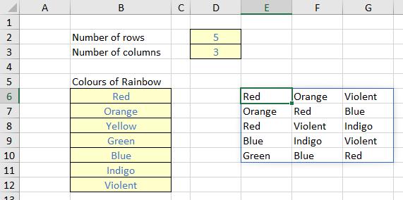
Imagine, for reasons best known to myself, I wanted to generate an array of colours of the rainbow (albeit with the final colour, ahem, slightly amended).  In the image above, I have specified the number of rows (cell D2) and the number of columns (cell D3) in my array, and listed the colours in cells B6:B12 inclusive.

The formula in cell E6 is given by

The first two arguments in this formula are D2 and D3, which refer to the number of rows and columns for the array to be generated respectively.  The final argument of MAKEARRAY is the LAMBDA, which must take two parameters, corresponding to the value generated by LAMBDA, namely:

• row: the index of the row
• column: the index of the column.

The calculation thus uses the non-dynamic array function RANDBETWEEN to generate an integer between one [1] and seven [7] to select from the list of colours of the rainbow, stipulated in cells B6:B12.  For example, if Excel generates the number 5, the value “Blue” will be chosen, etc.

Now it is true that existing functions could be used to achieve the same result, e.g.

This formula seems shorter and simpler, and indeed, may be the better option for this above illustration.  But that is exactly what this is – a simple example.  As more complex arrays need to be created, existing function counterparts may prove difficult, convoluted or impossible to construct – and this is precisely where MAKEARRAY and LAMBDA come in.

MAP

Ladies and gentlemen, may I welcome to the fore, Excel’s 500^th function – as agreed by fellow Excel Most Valuable Professional (MVP) Bill Jelen and yours truly. 

If you are giddy from this amazing fact, do be aware that the MAP function does not actually return a map!

Instead, it returns an array formed by mapping each value in the array(s) to a new value and applying a LAMBDA to create a new value accordingly.  It has the following syntax:

where:

• array1: this is a required argument and represents the (first) array to be mapped
• array2 and subsequent arrays: these are optional arguments and represent additional arrays to be mapped
• lambda: this is a required argument which represents a LAMBDA which must be the final argument and must have a parameter for each array passed or another array to be mapped.

In short, MAP transforms values.  Let’s return to my Melbourne temperatures data:

The formula

which returned the array

The problem is, these temperatures have all been provided in Celsius, which my co-author Chris doesn’t really understand.  If he sees a temperature of 25 degrees, he will be breaking out the gloves, bobble hat and duffle coat, whereas us Aussies will be heading for the beach. 

We need to convert – transform – this data to Fahrenheit, so our US colleagues may better understand.  All I need to do is wrap the above formula in a MAP function:

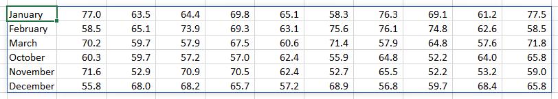
CONVERT(temperature, “C”, “F”) simply converts the variable temperature from degrees Celsius to degrees Fahrenheit.  This is wrapped in an IF(ISNUMBER()) check to ensure that we don’t try to convert text values (as this would cause an error): the IF statement leaves the value of temperature “as is” in this instance, and LAMBDA just wraps around all of this in order to declare the variable temperature “work”, so that MAP may do its work.

It’s true you could generate this result in stages, but the whole idea of these LAMBDA helper functions is to be able to create dynamic arrays in one fell swoop.

REDUCE

This penultimate function reduces an array to an accumulated value by applying a LAMBDA function to each value and returning the total value in what is known as the accumulator.  Its syntax is as follows:

where:

• initial_value: this is an optional argument and represents the starting value for the accumulator, i.e. the “running total” prompted by the lambda expression
• array: this is a required value and represents the array to be reduced
• lambda: this is also a required value and represents a LAMBDA function called to reduce the array, that consists of two parameters:
  • accumulator: the returned (aggregated) value from LAMBDA
  • value: a value from array.

Returning to our temperature example given by the Excel Table Temps:

we could count how many months in the 10-year period had an average temperature between 15 and 20 degrees Celsius as follows:

For each element of the Temps Table, defined by the LAMBDA function as value, the IF statement tests whether the temperature is between 15 and 20 degrees Celsius:

If this is true, one gets added to the running total (accumulator), so that a count is maintained.  The first argument of REDUCE – zero [0], the optional argument – simply specifies the starting value (initial_value) for the accumulator, which must be zero in order for the count to make sense.

Again, we could create a second array which performs a corresponding check for each cell and count the TRUE values, but this formula reduces the workload (i.e. it reduces the array of values to just one value by making use of the specified LAMBDA), allowing the computation to be performed once again without any helper stages.

SCAN

This final function scans an array by applying a LAMBDA to each value and returns an array that has each intermediate value.  The syntax is as follows:

where:

• initial_value: this is an optional argument and represents the starting value for the accumulator, i.e. the “running total” prompted by the lambda expression
• array: this is a required value and represents the array to be scanned
• lambda: this is also a required value and represents a LAMBDA function called to scan the array, that consists of two parameters:
  • accumulator: the returned (aggregated) value from LAMBDA
  • value: a value from array.

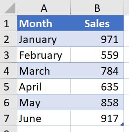
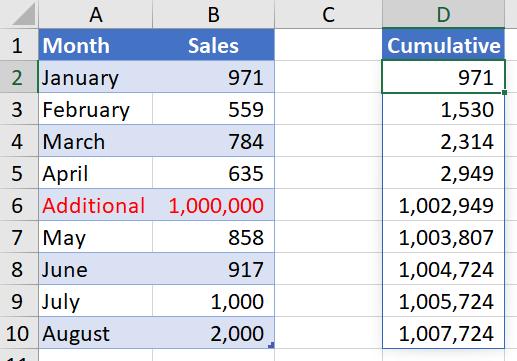
As a simple example, let’s consider a common problem when working with structured references, i.e. Excel Tables.  Imagine I have the following sales for the first six months of the year:

I might wish to create a running total of these sales.  One way I have seen people do this is as follows:

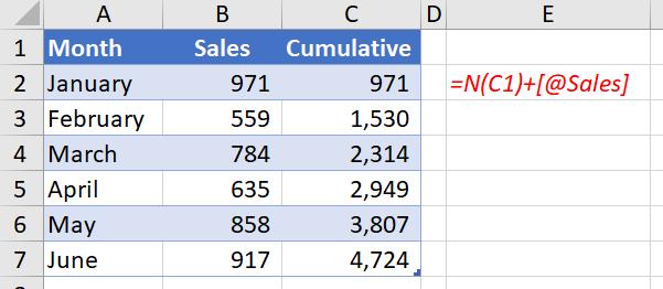
This is a horrible “hotch potch” of a formula:

It mixes Excel cell referencing (cell C1, because you cannot refer to a value for a different record simply in an Excel Table), structured referencing ([@Sales]) and the N function, in order to treat the numerical value of text as zero [0] and therefore avoid #VALUE! errors when adding amounts together.

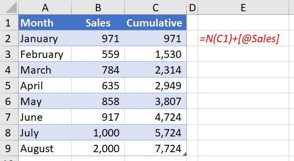
It seems to work if values are added:

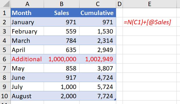
However, it all goes pear shaped when values are inserted:

This is where SCAN comes to the rescue.  Assuming the Table is also called Sales (not just the field in column B), we can create the formula

SCAN “scans” the array (i.e. the Excel Table Sales) by applying a LAMBDA to each value.  It then returns an array of results corresponding to the accumulator value returned by the LAMBDA.  As stated above, SCAN takes two parameters:

• accumulator: the initial value returned by SCAN and each LAMBDA call
• value: a value from the supplied array.

As above, the initial_value is zero [0] so that the running total calculates correctly.

Word to the Wise

These functions will not be for everyone, in more ways than one.  There are two key points:

1. The concepts discussed here revolve around the notion of lambda functions, which may not be relevant to all users, especially for those that use Excel for “simple” tasks.  But don’t let it scare or deter you from experimenting with these functions
   
   
2. These new functions are only available presently to c. 50% of Office Insiders users running Beta Channel Version 2108 (Build 14312.20008) or later on Windows, or Version 16.52 (Build 21072100) or later on Mac.  The LAMBDA function is now available to Office Insiders running Current Channel Preview Version 2107 (Build 14228.20154) or later on Windows, or Version 16.51 (Build 21071101) or later on Mac.