
New Data Types and FIELDVALUE Function Now Generally Available (Sort Of)
25 September 2018
We first mentioned this in May as a Preview feature, but now it’s being rolled out to all users of Excel in Office 365 (in the English language only) starting from late September.
Excel has always been great at helping people make the most of numbers. However, now Excel can do even more: it can recognise real-world concepts, starting with Stocks and Geography. This new AI-powered capability turns a single, flat piece of text into an interactive property (known as an “entity”) containing layers of “data rich” information. For instance, by converting a list of countries in a workbook to “Geography” entities, customers can weave location data into an analysis of their own data. This will be the start of new data types over time, allowing Excel’s rows, columns, cells, logic engine and tools to be used to organise, analyse and reason over any combination of numbers and sophisticated entities. The Stocks and Geography data types are generally available today.
Here’s a brief summary of these two new data types (first detailed in our May newsletter):
Data Type 1: Stocks
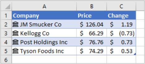
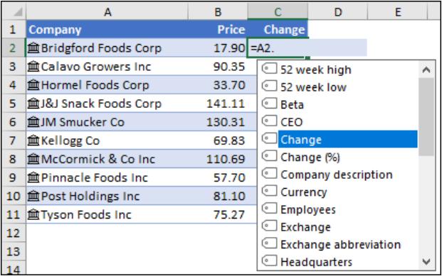
In this graphic, the cells with company names in column A contain the ‘Stocks’ data type. You may tell this because they have this icon . The ‘Stocks’ data type is connected to an online source that contains more information. Columns B and C are extracting that information. Specifically, the values for price and change in price are getting extracted from the ‘Stocks’ data type in column A.
Data Type 2: Geography
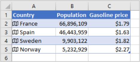
In this example, column A contains cells that have the ‘Geography’ data type. This time, the icon indicates this. This data type is connected to an online source that contains more information. Columns B and C are again extracting that information. Specifically, the values for population and gasoline price are getting extracted from the ‘Geography’ data type in column A.
We are sure you can see how these data types might be useful. So how do you set it up? Assuming you have had your version of Excel 2016 updated, it’s as easy as, er, 1, 2, 3, 4, 5, 6…
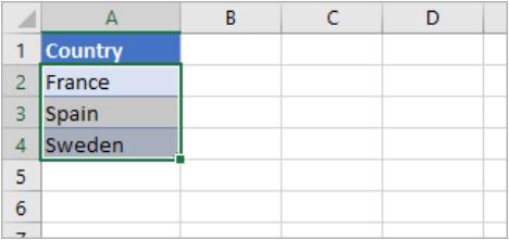
Step 1: Type Some Text
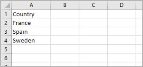
That’s right: just type some text in cells. In this example, we wanted data based on geography, so we typed country names. However, you could also have typed province names, territories, states, cities, etc. If you want stock information, similarly type company names, fund names, ticker symbols, and so on.
Step 2: Create a Table
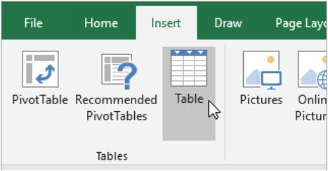
Although it's not required, it is recommended you create an Excel Table. This is so ranges may be extended readily and easily later, should you wish. Select any cell in your data and go to Insert > Table or use the keyboard shortcut CTRL + T. This will make extracting online information easier later on.
Step 3: Select Some Cells
Next, select the cells that you want to convert to a data type.
Step 4: Pick a Data Type

On the ‘Data’ tab, click either ‘Stocks’ or ‘Geography’.
Step 5: Icons Appear
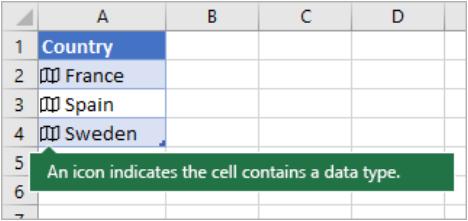
If Excel finds a match between the text in the cells and the online sources, it will convert your text to either the ‘Stocks’ data type or ‘Geography’ data type. You will know immediately if they have been converted since they will have the icon for stocks and the icon for geography.
Step 6: Add a Column
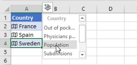
Click the ‘Add Column’ button , and then click a field name to extract more information, such as ‘Population’.
If you see the symbol instead of an icon, then Excel is having difficulty matching your text with data in Microsoft’s online sources. Go back and review your data. Correct any spelling mistakes and when you press ENTER, Excel will do its best to find matching information. If this does not work, click and a ‘Selector’ pane will appear. Search for data using a keyword or two, choose the data you want and then click ‘Select’. That’s it!
How to Write Formulae that Reference Data Types
You can use formulae that reference linked data types. This allows you to retrieve and expose more information about a specific linked data type. For example, consider the linked data type, Stocks, used in cells A2:A11 below. In columns B and C, there are formulae that extract more information from the ‘Stocks’ data type in column A, viz.
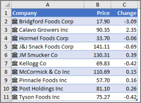
In this example, cell B2 contains the formula =A2.Price? and cell C2 contains the formula =A2.Change. When the records are in a Table, you can use the column names in the formula instead. In this case, cell B2 would contain the formula =[@Company?].Price and cell C2 would contain =[@Company].Change. The additional benefit is that these formulae would automatically copy down too.
Some tips for when you start playing with these two new data types:
- as soon as you type the dot operator (.) after a cell or column reference, Excel will present you with a formula AutoComplete list of fields that you can reference for that data type. Select the field you want from the list or type it if you know it
- data type field references are not case sensitive, so you can enter =A2.Price, or =A2.price
- if you select a field that has spaces in the name, Excel will automatically add brackets ([ ]) around the field name, e.g. =A2.[52 Week High]
- the FIELDVALUE function can also be used, but it is recommended only for creating conditional calculations based on linked data types.
This last point is a nice lead into the other new item…
The FIELDVALUE Function
You can use the FIELDVALUE function to retrieve field data from linked data types like the ‘Stocks’ or ‘Geography’ data types. There are easier methods for writing formulae that reference data types (see above), so the FIELDVALUE function should be used mainly for creating conditional calculations based on linked data types.
Similar to the new data types, this brand-new function is being made available to customers on a gradual basis over several days or weeks. It will first be available to Office Insider participants and later to Office 365 subscribers. If you are an Office 365 subscriber, make sure you have the latest version of Office or you may not get the update when it’s your turn.
Technical details
Syntax
=FIELDVALUE(value, field_name)
The FIELDVALUE function syntax has the following arguments:
- value: this is the cell address, table column or named range that contains a linked data type
- field_name: this is the name or names of the fields you would like to extract from the linked data type.
Description
The FIELDVALUE function returns all matching fields(s) from the linked data type specified in the value argument. This function belongs to the Lookup & Reference family of functions.
Examples
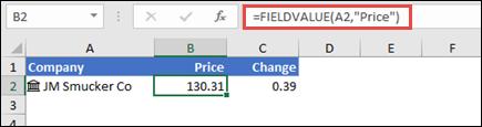
In the following basic example, the formula, =FIELDVALUE(A2,"Price") extracts the Price field from the ‘Stock’ data type for the “internationally-renowned” JM Smucker Co.
The next example is a more typical example for the FIELDVALUE function. Here, we’ve used the IFERROR function to check for errors. If there isn't a company name in cell A2, the FIELDVALUE formula returns an error, and in that case, displays nothing (""). However, if there is a company name, then we want the formula to retrieve the Price from the data type in A2 with =IFERROR(FIELDVALUE($A2,B$1),"").
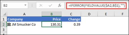
Note that the FIELDVALUE function allows you to reference worksheet cells for the field_name argument, so the above formula references cell B1 for Price instead of manually entering "Price" in the formula.
Word to the Wise
If you try to retrieve data from a non-existent data type field, the FIELDVALUE function will return the new #FIELD! error. For instance, you might have entered "Prices", when the actual data type field is named "Price". Double-check your formula to make sure you've used a valid field name. If you want to display a list of field names for a record, select the cell for the record and press CTRL + SHIFT + F2.
Happy playing with your new toys!
FIELDVALUE will be detailed in our blog series A to Z of Excel Functions in due course. You can find out about other functions in our current list here. And don’t forget to subscribe to our newsletter (form at the bottom of any SumProduct web page) to keep up to date with all that’s new, weird and wonderful in Excel.