
Manual versus Automatic?
Introduction
As a professional modeller, FCA and Excel MVP Liam Bastick highlights some of the more useful functions for financial modelling / Excel spreadsheeting. Forecasting is an integral part of most accountant’s work and here he considers two ways of extrapolating objectively.
Objective Forecasting
Let’s face an ugly truth in the world of finance / accounting. It’s the operational managers at the coalface who have the best understanding of likely demand and expected costs, yet many do not have the necessary tools or financial skills to forecast to the level that senior management requires. Similarly, most analysts do have these skills but may not be close enough to the front line to be able to understand operations sufficiently.
Operational managers and analysts need to work together to improve forecasting. That goes without saying and is never a problem in reality as the two sides work beautifully together, skipping off into the sunset hand in hand after a productive day in the office, understanding each other’s needs and issues.
Yeah, right. If you believe that you’re probably a Board Director…
Meanwhile, back on Planet Earth, often we find managers and analysts in a state of “co-operational flux” (a new term I have just invented). Managers sometimes feel accountants / analysts request forecasts from scratch: do they have either the time or skills to prepare a zero-based budget, whereas the analysts feel if they spend time preparing the base budget it is then torn apart by their operational counterpart. The art of war / budgeting: don’t you just love it?
There is a need for objective forecasting. By this, I mean something that can be constructed simply such that if anyone follows the same process they will get the same figures. This needs to be a mechanical, objective process. This way, analysts may prepare this data in moments without feeling emotionally attached to the outputs. Furthermore, operational managers can review the trend and state where future numbers are wrong and all they need to do is explain the variation, i.e. undertake incremental budgeting. There is no need to disagreements or confrontation: both parties may work together as a team. Simple!
Wow, is that the longest preamble for an Excel blog ever..?
I wanted to set the scene for having a simple mechanical approach for budgeting. Using my attached Excel file (below), let’s take a look at ways Excel can do this for you. Imagine I have some historical data:
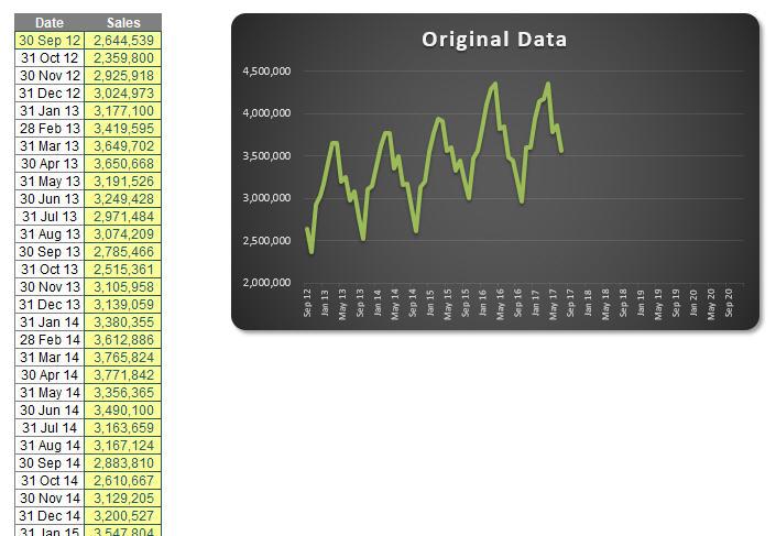
Now let’s be honest, anyone who has historical data looking this perfect should be referred to the auditors, but hey, this is for illustration purposes. I have data from September 2012 to July 2017. I want to extrapolate it until the end of 2020 (I want 2020 foresight!).
There are several functions that can help us here, with one of the simplest being TREND. TREND(known_y’s,known_x’s,new_x’s,[constant]) projects assuming that there is a relationship between two sets of variables x (independent variable – here, the dates) and y (dependent variable – the sales), through a formula y = ?x + c, i.e. the equation of a straight line (? is the gradient of the line and c is the y-intercept).
Before you disregard linear regression, bear in mind many non-linear relationships can become linear ones by taking logarithms of the variables, for example. However, this won’t always work.
Here, time is our independent variable (x) and sales is our dependent variable (y). We only specify the constant if we want to force c in the equation (not common – it will usually be left blank). Similarly, it’s preferable to leave constant blank in the TREND function. For example:
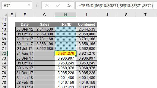
Here, we can extrapolate the data using the TREND function viz.
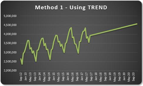
Ladies and gentleman, you may have heard of hockeystick projections; well, let me now present you with the swordfish. You extrapolate linearly, you get a straight line. Now who would like to present that projection to their senior management team?
This isn’t good enough. We need to identify the cyclicality of the data. It appears to go through a cycle once every 12 months. This might not always be the case, but the concept remains the same even if the periodicity is not annual.
I want to calculate a periodic growth rate objectively. There’s various ways I can do this. You might argue with me. That’s fine. Feel free to write a brief note and send it to someone who cares. That’s the problem here – it’s subjective until your organisation defines how it is to be measured. Then, everyone follows that process and it becomes objective.
In my example, I am going to compare the sum of the sales over the 12 months ending 31 July 2017 with the forecast sales as calculated using TREND over the 12 months ending 31 July 2018:
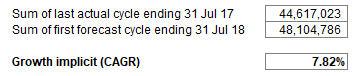
It is this percentage I will use to grow the forecasts (note the attached Excel file allows for different periodicities as long as the cycle remains constant).
I then grow each period’s value by its corresponding value in the previous period by this percentage (7.82% here). This gives me a much better chart:
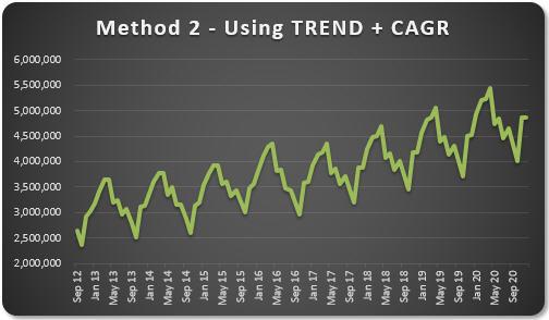
That looks much better. With practice, this approach doesn’t take that long to prepare. Numbers may be varied from this forecast with the operational manager only having to explain these deviations. It makes life easier all round.
Once the method of assessing inferred growth rates based upon the TREND function have been agreed and what normalisations to historical data should be input, the process becomes much more straightforward. Of course, this method should be used for all forecast inputs separately and not just on their aggregation, otherwise confusion occurs due to sales mix changes, new products, cut-off periods, etc.
But there is an even faster way – if you happen to have Excel 2016…
Exponential Triple Smoothing (ETS) sounds like a dairy process, but it actually uses the weighted mean of past values for forecasting. It’s popular in statistics as it adjusts for seasonal variations in data, like in the example above. For those who really need to know, Excel uses a variation of the Holt Winters ETS algorithm, although to be honest, I think you should get out more.
In Excel 2016, ETS has gone “native”, i.e. it is a standard feature. This includes both a set of new functions such as FORECAST.ETS and other supporting functions for additional statistics. Your dataset does not need to be perfect, as the functions will accommodate up to 30% missing data.
But don’t worry about using these functions. Simply highlight the actual data and click on the ‘Forecast Sheet’ button in the ‘Forecast’ group of the ‘Data’ tab of the Ribbon (ALT A + FC):
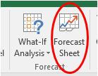
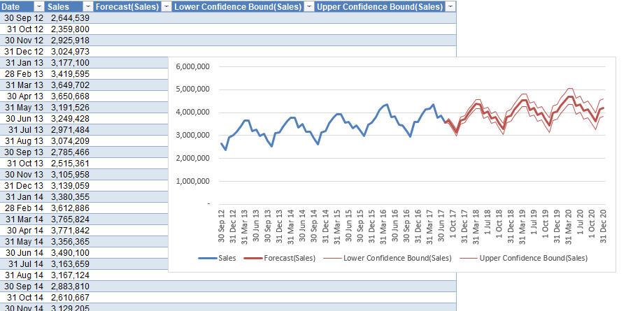
All you need to do is specify the final forecast period at the prompt and that’s it. It produces a raw data sheet, together with confidence intervals (to demonstrate potential spread in the forecast error), which looks something like this:
Manual versus automatic?
- The “manual” method, using TREND, assumes some linear relationship (possibly at a derivative level) and requires some initial subjectivity regarding the normalisations of actual data and how to determine what growth rate to use over what duration. Once it has been agreed, it becomes a simple process both to understand and maintain.
- The “automatic” method using the Forecast Sheet works it all out at the press of a button, after normalisations to historical data have been made. However, it’s not all peaches and cream: it’s only available in Excel 2016, it’s quite “black box” to many and could you really explain to your line manager what Exponential Triple Smoothing is?
The jury remains out: whatever you decide, for your own sanity, I recommend an objective forecasting approach.