
Evaluating EVALUATE
Some functions just shouldn’t be talked about in polite circles. This article explores what appears to be one of the most bizarre functions in Excel – the little-known EVALUATE. By Liam Bastick, director with SumProduct Pty Ltd.
Query
A colleague has mentioned Excel’s EVALUATE function to me but I can’t get it to work. Any advice..?
Advice
Not all functions are documented in Excel. Some seem to have been swept under the rug ne’er to be discussed for fear of Microsoft retribution. Try looking up the EVALUATE function in Excel’s Help, for instance. In fact, try using it (“That function is not valid”)! EVALUATE is possibly one of the most bizarre functions in Excel – yet it is a useful one if you can work out how to use it…
Consider the following complex spreadsheet:

EVALUATE essentially converts text strings into formulae that can be, er, evaluated. Theoretically,
=EVALUATE(A1&A2&A3)
would be EVALUATE(1+2) which is 3. All good, except it doesn’t work unless you use it via a range name definition.
Range names have been discussed in another article (see Naming Names for further information). Assuming the worksheet is imaginatively named ‘Sheet1?, the trick here is to define a range name (CTRL + F3, then click on ‘New…’ button) as follows:
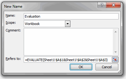
Note that you must use the sheet names for this to work. Now, if you type
=Evaluation
into cell A4, say, suddenly EVALUATE (cited in ‘Refers to:’ of the ‘New Name’ dialog box, above) comes to life and provides the expected result (here, 3). Changing the contents of cells A1, A2 and A3 to ’4?, ‘x’ and ’7? respectively will change the result to 28, as expected. It is in this manner that EVALUATE has a passing resemblance to INDIRECT (see Being Direct About INDIRECT).
With a little experimentation, you will see that the Evaluation range name can be used to evaluate different cells in the same spreadsheet simply by removing the anchoring (i.e. remove some or all of the $ signs).
Readers may not quite see how this is useful, but consider the following example, which I cannot take credit for. The following idea has been created previously by fellow Excel MVPs Stephen Bullen and was then revamped by Jan Karel Pieterse.
Plotting a Chart with No Data Points
There are occasions when we need to plot charts. Sometimes, we plot actual data in order to ascertain trends and in this particular instance, we would need to create the chart from the data recorded. However, on other occasions, we will be considering existing formulae in order to create a chart. It is this scenario which this approach can help with.
However, let’s back up first. In a simple scenario, we would plot a chart as follows:
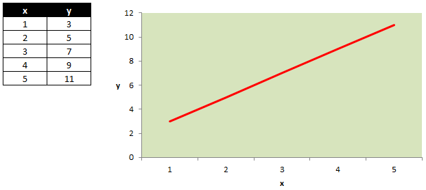
In this simple illustration of y = 2x + 1, we define x as our independent variable (the value we can control) and y as the dependent variable (i.e. the result). For example, we may spend $1,000 on marketing (x) and generate additional sales of $3,000 (y).
The question is, can we generate the chart without manufacturing the supposedly necessary data table?
To show this is indeed possible, I will exploit a little-known fact, that when a defined name is used to name a formula this formula will be an array formula by default (array formulae have been discussed previously in Array of Light).
As in the illustration above, we first need to generate an automatic list of x values. This can be done as follows.
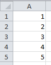
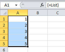
Consider the range A1:A5, viz.
I could name this range List using a method similar to the approach detailed above. Alternatively, I could generate this list automatically as follows:
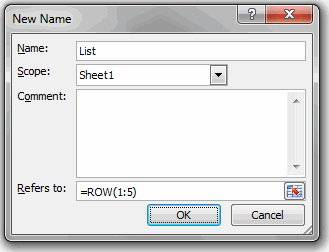
Now, if we enter =List as an array formula (CTRL + SHIFT + ENTER) into cells A1:A5 we get the same data as above, but automatically.
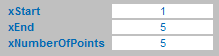
I need to construct my data more flexible. Essentially, I want an incremental set of data points to be generated by specifying a starting value (xStart), an end point (xEnd) and the total number of data points (xNumberOfPoints):
Using the OFFSET function (see Onset of OFFSET), we can generate the list as follows:
=ROW(OFFSET(Sheet1!$A$1,0,0,xNumberOfPoints,1))
However, this doesn’t take into account the start and end points. If we define xRange as the value xEnd – xStart, we can construct the data set
x := xStart+xRange/(xNumberOfPoints-1)*
(ROW(OFFSET(Sheet1!$A$1,0,0,xNumberOfPoints,1))-1)
I call this x to be consistent with my explanations above, rather than List used in the simple example. In order to get this to work properly in Excel, you should ensure that this range name is sheet specific, e.g. we will give this formula the range name Sheet1!x.
I am halfway there. Now that I have an automatic way of generating a list of data points for my independent (x) variable, I need to create the results (y). To do this, I first need to define the formula that will generate the results:

Formulae should be written without the equals sign using functions Excel recognises. Note that the variable must be x, otherwise this whole process will not work. Also, to make the formulae more transparent, I have named the formula cell – very imaginatively, I might add – Formula.
As in my first example, I will use EVALUATE:
y := EVALUATE(Formula)
As with the range name for x, this range name must be defined sheet specifically (e.g. Sheet1!y).
Unfortunately, it’s not as ‘simple’ as this. EVALUATE does not seem to work for Excel’s built-in functions, like SIN used in the illustration above. If constructed as above, the reader will note the same value is generated for y, regardless of the value selected for x. To circumvent this issue, I employ the following trick:
y := EVALUATE(Formula&”+0*x”)
By adding this ‘zero text string’, EVALUATE will now work as envisaged.
The attached Excel file includes a working version of this example.
Word to the Wise
EVALUATE is actually an old xl4 macro function (i.e. pre-VBA). These old functions are still recognised if and only if they are used inside Excel range names, and therefore, more experienced (older?) users may wish to resurrect other long-forgotten functions in a similar contrived manner too.