Dynamic Data Validation

28 August 2020

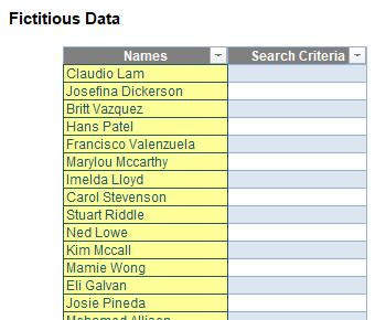
Here is a common problem that has been a pain point for modellers for many years.  Imagine you had a dataset of customer names (say):

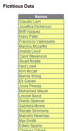
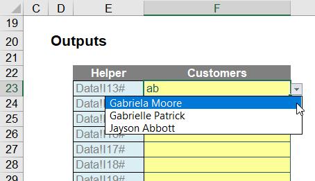
In the example in the attached workbook, I have put 200 random names in (but this method will work for up to 10,000).  What I want to do is create an output sheet where I can select a name from a dropdown list, but with it filtering for any letters I have already typed into the cell, viz.

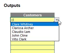
Do you see how I have typed in “cl” and it has returned any names with “cl” in the name – including names not necessarily starting with these two letters (e.g. John Cline).  Furthermore, if I type a further letter, say “o”, this then becomes:

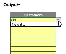
How good would that be when you have long lists, unordered, with potential duplicates?  No more endless scrolling – simply type in several key letters and choose from a filtered selection instead.  Accountants, analysts, managers and modellers have been striving for this sort of functionality in Excel for years.

Previous Solutions

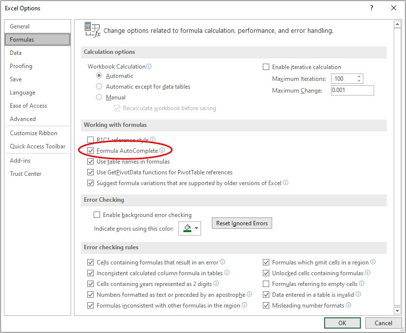
People have developed VBA solutions or used Excel’s ability to AutoComplete.  For example, if you ensure Formula AutoComplete is enabled (File -> Options, or ALT + T + O) by checking the appropriate box in the ‘Working with formulas’ section of ‘Formulas’,

You may then hide a complete list above your input cell (ensuring there are no gaps and start typing):

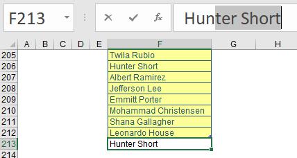
Here, I started typing the name “Hunter Short” into cell F213.  Once I typed the third letter in, Excel was ready to AutoComplete, as there was only one option remaining.  This is one option, but:

• It will not work with lists containing duplicates
• It assumes you are typing the first letters of the name in
• You have to replicate this list immediately above the input cell(s)
• It only displays once Excel has ruled out all other alternatives.

This is not ideal – so I shall stick with my plan instead.

New Solution

This solution will only work in Office 365 as it relies on the new feature, dynamic arrays.  You might think I am being a little niche in this instance.  However, if you do not have Office 365, keep reading.  This might convince you it’s time to make the switch.

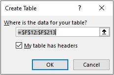
To start, I want to turn my data table, which I will assume is on a worksheet called Data, into an Excel Table.  I highlight the table and choose Table from the Tables group on the Insert tab of the Ribbon (CTRL + T).  Since the first row is the heading, I ensure the ‘My table has headers’ check box is ticked in the ‘Create Table’ dialog:

As you will see later, creating a Table is like a double-edged sword: it is useful as it will allow us to add more names to the list and the range will automatically extend, but it will cause us headaches elsewhere.

Having named the table ‘Customers’ in the ‘Table Design’ tab, I add an input column to my Table:

I can now start to build up my helper formulae.  The first function I am going to call upon is SEARCH. 

SEARCH(find_text, within_text, [start_number]) is a search function which is not case sensitive but does allow for wildcard characters.  It seeks out the first instance of a character or characters (typed in inverted commas) in the within_text text string.  The start_number argument is optional (hence the square brackets in the syntax) so that the first few characters in a text string may be ignored.  If the find_text cannot be located within within_text, the error #VALUE! is returned.

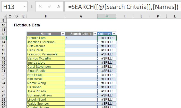
As in the image (below), I add a formula, but I exclude it from the Table by leaving an empty column between them, viz.

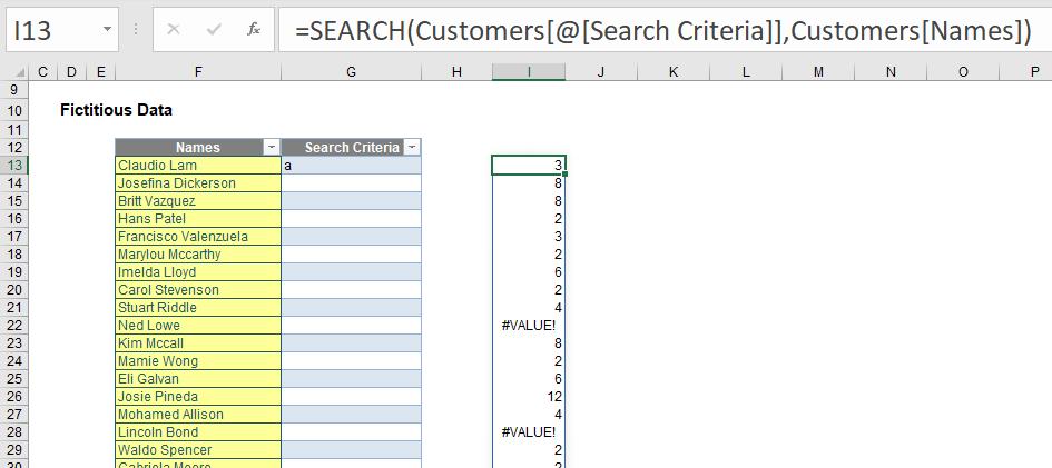
I will explain why this formula is not incorporated into the Table in a moment.  However, let’s first take a look at the formula which was typed into cell I13 only:

Customers[@[Search Criteria]] is the structured referencing syntax (i.e. how formulae work when references are from within an Excel Table) stating the Search Criteria item (sic) for that row.  This is what the @ symbol denotes – it’s not the Table’s Twitter handle.  In this case, this is cell G13, where I have typed in “a”.

Customers[Names] denotes the entire Names field.  Presently, this is represented by cells F13:F212 (i.e. 200 records) in my example.  However, if I were to add names to the bottom of the list, the range would extend automatically.  This is why I put this data in a Table: my formula is flexible.

If I had simply referred to the first row rather than the entire range, the SEARCH formula would have sought the character “a” in cell F13 – “Claudio Lam” – and returned the position of the first “a”, which would be 3 (third character).  However, I did it for the entire range, so this formula spilled: it added formulae down the entire column to match the length of the source argument and found the “a” in each row’s entry of Customers[Names].  This is what Office 365 will do (if you have Office 365 and it doesn’t, be patient, the update is very close).  You have created a dynamic array: it’s dynamic as the formula will extend / contract automatically as the source data length changes.

The reason I have not included this formula in the Table (which would seem to make more sense) is as follows.  Let’s imagine I had:

In this instance, the formula would have simplified because there is no reason to specify the Table name (Customers).  However, it doesn’t work.  The spill feature is not supported in Excel Tables – hence the double-edged sword I was referring to earlier – so this formula must be excluded from the source Table.  That will be a source of frustration later (oh yes, I do like to keep you on tenterhooks).

Returning to our current situation, 

do you see two of the entries in my extract (rows 22 and 28) return #VALUE! errors?  This is what happens when there is no “a” (in this example) in these text strings (“Ned Lowe” and “Lincoln Bond” respectively).  I don’t care where my “a” occurs, only that it occurs; further, I wish to remove my errors too.

Therefore, I use the ISNUMBER function.  One of 12 IS functions, this one is best suited here as it filters between numbers (TRUE) and everything else (FALSE) – including errors:

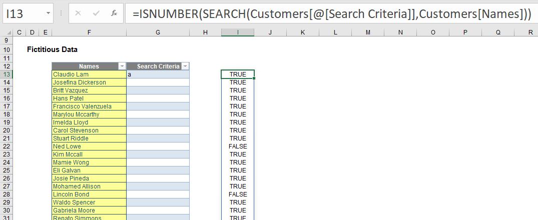
I could now filter on column I to produce a list in column F of those names which contain the letter “a” only.  However, I don’t want to do it this way.  I want to formulaically filter it, so I use the function new to Office 365 (which supports and creates dynamic arrays), FILTER.

FILTER Function

The FILTER function will accept an array, allow you to filter a range of data based upon criteria you define and return the results to a spill range.

The syntax of FILTER is as follows:

It has three arguments:

• array: this is required and represents the range that is to be filtered
• include: this is also required.  This specifies the condition(s) that must be met
• if_empty: this argument is optional.  This is what will be returned if no data meets the criterion / criteria specified in the include argument.  It’s generally a good idea to at least use “” here.

For example, consider the following source data:

It is simple to FILTER:

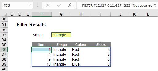
Here, in cell F36, I have created the formula

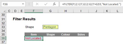
F12:I27 is my source array and I wish only to include shapes (column G12:G27) that are ‘Triangles’ (specified by cell G33).  If there are no such shapes, then “Not Located.” is returned instead.  To show this, I will change the shape as follows:

Returning to Our Solution

Therefore, let me use the following formula:

This merely builds on the last ISNUMBER calculation (which is the criterion), applying it to the field Customers[Names], with “No data.” returned should there be no matching results.  Having modified my input requirements from “a” to “au” (feeling Australian today), my calculation would appear as follows:

My list of TRUE and FALSE entries is no more, and has been replaced by the names that match the criterion (must contain “au”).  It’s starting to come together now.  Some of you might think you now have your data, but you can do better by ensuring there are no duplicate entries and sorting the data.  This requires two functions: UNIQUE and SORT, both new to Office 365 and both supporting the brave new world of dynamic arrays.

UNIQUE Function

Bizarrely, UNIQUE details distinct items (i.e. provides each value that occurs with no repetition) and also it can return values which occur once and only once in a referred range.  I will be focusing on the former use here.

The UNIQUE function has the following syntax:

It has three arguments:

• array: this is required and represents the range or array from which to return unique values
• by_column: this argument is optional.  This is a logical value (TRUE / FALSE) indicating how to compare.  If you wish to compare by row, the argument should be FALSE or omitted (since this is the default).  To compare by column, you will need to select TRUE
• occurs_once: this argument is also optional.  This requires a logical value too:
  • TRUE: only return unique values that occur once
  • FALSE: include all distinct values (default if omitted).

It’s probably clearer with an example.  Consider the following source data:

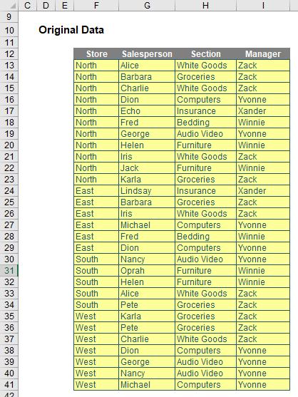
I can derive the unique items in each list:

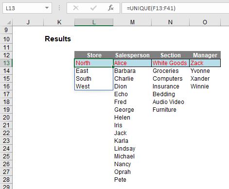
In cell L13, I have simply typed

No optional arguments; everything in default.  This has simply listed each store that appears; if “North” and “North ” (extra space) were there, then both would appear.  UNIQUE is not case sensitive though and each entry would appear as it first occurs reading down the range F13:F41. 

SORT Function

The SORT function sorts the contents of a range or array:

It has four arguments:

• array: this is required and represents the range that is required to be sorted
• sort_index: this is optional and refers to the position of the row or the column in the selected array (e.g. second row, third column).  99 times out of 98 you will be defining the column, but to select a row you will need to use this argument in conjunction with the fourth argument, by_column.  And be careful, it’s a little counter-intuitive!  The default value is 1
• sort_order: this is also optional.  The choices for sort_order are 1 for ascending (default) or -1 for descending.  It should be noted that you might not want to hold your breath waiting for ‘Sort by Color’ (sic), ‘Sort by Formula’ or ‘Sort by Custom List’ using this function
• by_column: this final argument is also optional.  Most people want to sort rows of data, so they will want the value to be FALSE (which is the default value if not specified).  Should you be booking your mental health check, you may wish to use TRUE to sort by column in certain instances.

Again, it’s simple.  Consider the following data:

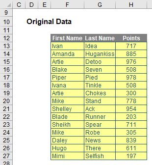
Sorting the ‘Points’ column in order is easy as this:

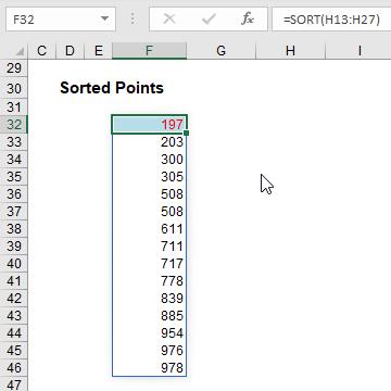
All you have to do is type =SORT(H13:H27) into cell F32.  That’s it.  However, do note that the duplicates are repeated; there is no cull.  That’s why it is needed here alongside UNIQUE.

Returning to Our Solution Again

Here, I need to remove duplicates and sort my data.  It does matter the order I perform these calculations: {2, 1, 3} is easier to sort than {1, 2, 1, 2, 2, 1, 3, 3, 1, 1, 2, 3, 2, 1}.  I should remove duplicates first, then sort. 

This is an important mindset to get into: working with dynamic arrays can mean you start taking for granted some rather voluminous but unnecessary tasks otherwise.  Putting functions in the wrong order can make the difference between a one and a 10 second calculation.  Therefore, my formula extends to

Now comes a trick: instead of having this list propagate vertically, I wish it to fill horizontally.  I can achieve this with the TRANSPOSE function:

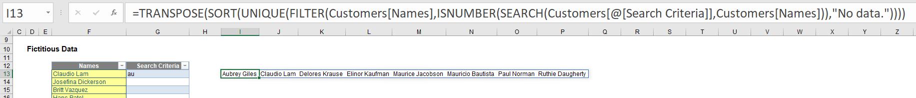
Yes, the graphic is tiny – but it’s more about the concept than the detail here.  My list now extends across the row, which means I can now copy my formula down column I, viz.

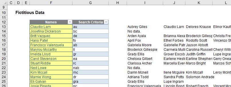
Hopefully, my idea is becoming clearer.  I can use the criteria typed in column G to generate the spilled horizontal lists in column I onwards.  Therefore, if I change the contents of column G to reference the data in other cells where I want my output dropdown boxes to be, I can then create lists for these cells based upon column I onwards.

Hence, on a separate worksheet, I now undertake some workings:

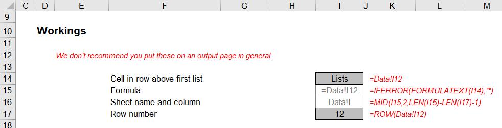
It might not seem obvious what I am doing, so allow me to explain.  I want to set a reference cell immediately above where the formula for my first dynamic list is (i.e. cell I13 on the Data worksheet).  This is so that I can set a base cell for my source data.

If you cannot follow the formula in cell I14, then I humbly suggest Excel may not be for you; cell I15 then displays the formula in cell I14 using FORMULATEXT (with an error trap in case of unforeseen issues).  This has then catered for any change in cell for the base cell, or a change of sheet name.

I will skip a formula momentarily: the calculation in cell I17 (=ROW(Data!I12)) merely generates the row number, so that the formula in cell I16 is

which is not as easy to understand as it could be!

The function LEN determines the length of a text string.  Therefore:

• LEN(I15) determines the length of =Data!I12, which is nine (9) characters
• LEN(I17) determines the length of the row number (12), which is two (2) characters
• LEN(I15)–LEN(I17) is therefore the length of =Data!I (no row number reference), which is seven (7) characters
• LEN(I15)–LEN(I17)-1 is one character less.  This is not to get rid of the column reference (I) but actually the equals sign (=) at the beginning.  This will become clearer shortly.

MID(text, start_number, n) extracts n characters from the referenced text string starting with the character in position start_number.  Thus,

will extract six (6) characters from the text string in cell I15 (=Data!I12), starting at the second character (i.e. ignoring the equals sign).  This gives the result Data!I. 

This all does beg the question, so what?

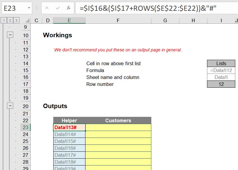
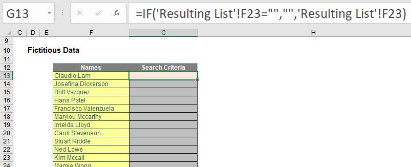
I want to create a set of customisable drop-down lists starting in cell F23.  To assist, I add a Helper column in column E:

Cells F23 down are then referred to back on the Data sheet:

This will now drive my dynamic lists in column I onwards.

Returning to the output sheet, the formula in cell E23 needs explanation:

Through the concatenation operator (&), this formula joins up the text in cell I16 (Data!I) with a number that starts with 12 (cell I17) and adds on the number of rows from row 22 ($I$17+ROWS($E$22:$E22)).  This is then joined to “#” to form

Data!I13#

The # symbol is known as the spilled range operator and denotes the full range (given that it is dynamic and may vary in size).  Next, I create a dropdown list in cell F23.  To do this, I select this cell, then go to ‘Data Validation’ in the ‘Data Tools’ group of the Data tab of the Ribbon (ALT + D + L),

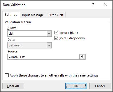
On the Settings tab of the resulting dialog box, I choose to List from the ‘Allow:’ selection and initially, I could type in =Data!I13# as the source (this has to be typed as # will not appear automatically by selecting a range).  If I selected the entire possible range instead this would make the data validation lists unnecessarily large and show many blank rows needlessly. 

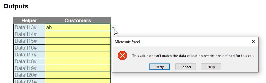
This would give an error if I tried to start typing something:

Therefore, I need to go back to the Data Validation dialog and click on the third tab, ‘Error Alert’:

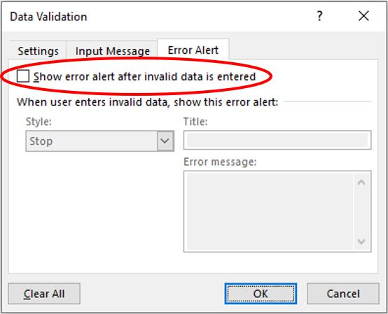
I must uncheck ‘Show error alert after invalid data is entered’.  After clicking OK, it would then work as envisaged.  

However, I would have to create each dropdown individually (due to the #), which would be a pain if I were to add 200 dropdown boxes (say).  Ain’t nobody got time for that.  Therefore, I turn to one of the most divisive functions in Excel…

INDIRECT Function

Excel’s INDIRECT function allows the creation of a formula by referring to the contents of a cell, rather than the cell reference itself.  The INDIRECT(ref_text, [a1]) function syntax has two arguments:

1. ref_text: this is a required reference to a cell that contains an A1-style reference, an R1C1-style reference, a name defined as a reference or a reference to a cell as a text string.  If ref_text is not a valid cell reference, INDIRECT returns the #REF! error value.  If ref_text refers to another workbook (an external reference), the other workbook must be open.  If the source workbook is not open, INDIRECT again returns the #REF! error value
2. [a1]: this is optional (hence the square brackets) and represents a logical value that specifies what type of reference is contained in the cell ref_text.  If a1 is TRUE or omitted, ref_text is interpreted as an A1-style reference (e.g. A1, C5, J199).  If a1 is FALSE, ref_text is interpreted as an R1C1-style reference. 

Essentially, INDIRECT works as follows:

In the above example, the formula in cell H18 (the yellow cell) is

With only one argument in this function, INDIRECT assumes the A1 cell notation.  Note that the value in cell H11 is H13, so this formula returns the value / contents of cell H13, i.e. 187. 

Completing Our Solution

Now do you see why I have that Helper column in column E?  I modify my data validation list (ALT + D + L) one final time:

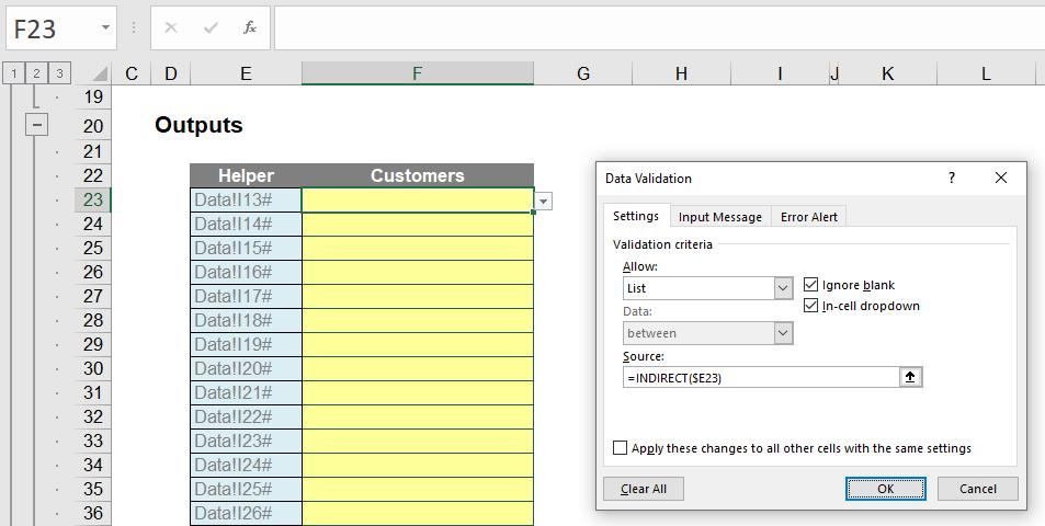
I have replaced =Data!I13# with =INDIRECT($E23) – that is the equivalent of =Data!I13#.  This step allows the data validation to be copied down the range, viz.

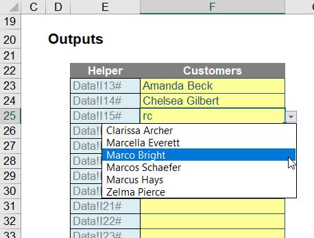
Success! The attached Excel file provides the full example for review.

Word to the Wise

This article has only required access to dynamic ranges, data validation, creating a Table, structured referencing, three operators (#, & and =), three text functions (SEARCH, LEN and MID), an array function (TRANSPOSE), three dynamic array functions (FILTER, UNIQUE and SORT) and one non-auditable function (INDIRECT).  I think it’s my most comprehensive example yet!

If you have a query for the Spreadsheet Skills section, please feel free to drop Liam a line at liam.bastick@sumproduct.com or visit the SumProduct website.