Debt Sculpting

Introduction

As a professional modeller for more years than he’d care to admit FCA Liam Bastick highlights some of the ways to avoid the need to use macros in financial modelling / Excel spreadsheeting.  This article highlights how accountants can get rid of common macros by organising their spreadsheets better…

A Debt to Repay

Debt is a key element of most financial models.  Clearly, if debt is to be borrowed it must be repaid at some point.  This associated debt repayment profile is seldom arbitrary and it is usually forecast to meet certain criteria.  I am going to discuss three common approaches here:

1. Debt Service Coverage Ratio (DSCR) approach;
2. Project Life Coverage Ratio (PLCR) approach; and
3. Loan Life Coverage Ratio (LLCR) approach.

I am not saying these are the only techniques in existence (optimum debt sizing and Weighted Average Cost of Capital (WACC) optimisation approaches are others), but hey, I have to draw the line somewhere.  Besides, even the most proficient modellers can make a terrible mess of the three approaches cited above.

Modellers often revert to macros to construct the appropriate debt repayment profile.  This is not usually necessary.  Key to calculations is the amount of cash available – known as the Cash Flow Available for Debt Servicing (CFADS).  Typically, this is the cash generated in the period (usually a calendar or financial year) prior to the debt principal and interest being paid (and any equity payments), but after tax has been accounted for excluding any shield on the interest repaid. 

Repayment calculations often get into a tangle leading to circular logic, chiefly for two reasons:

1. Interest is not calculated on the opening debt balance alone.  Drawdowns are often used to fund shortfalls caused by costs such as interest paid; repayments are subject to the cash available which is reduced by the amount of any interest paid.  Therefore, any reference to a balance or movement other than the opening debt for the period may cause circular logic in any formulae constructed.
   
   I have dealt with avoiding circularities when calculating interest on average balances before using algebra (please see here for further information).  Therefore, I won’t be discussing this here.  In any case, in many instances calculating interest on opening balances is acceptable (perhaps after making the periods shorter).
   
   
2. Tax is a key component of CFADS.  However, tax is based on Net Profit Before Tax, which is after Interest Expense.  Therefore, if CFADS is used without thought, interest will be a function of CFADS available, but CFADS is calculated after interest.  This can seem like an unavoidable circularity but this is simply not the case.

Therefore, many modellers will use macros to copy and paste as values the CFADS figure (and possibly the debt balances too) in order to avoid circularities.  This method may not generate the right answer and is simply not warranted.  It’s all about calculating CFADS suitably and I will use the attached Excel file as my example.

Let me start with a draft Cash Flow Statement:

For simplicity, I assume there is only an initial debt drawdown (cell J37).  All of the yellow cells here are inputs: grey cells depict further calculations – not yet made – have to be included.  So I suppose we had better get on with it!

Interest paid and debt repayments are our end products so let me come back to them later.  Given Interest Received forms part of the Tax Paid calculation, that will need to be computed, but there is one other item I need to calculate too.  Net Capital Expenditure is not a relevant expense item for tax purposes and needs to be “smoothed’ using depreciation instead of the figures in row 30 (above):

The formula in cell J66,

calculates the appropriate depreciation charge on a straight-line basis preventing any over-depreciation and allowing for the calculations to start in the right period using the counter in row 9.

Next, I need to calculate interest on the cash available.  Here, I have not concerned myself with overdraft fees, but it is simple to add these in.  I will concentrate merely on interest received on surplus cash. 

I will assume cash is received (not necessarily accrued) evenly over the period, so I will assume the average cash balance for the period is the midpoint between opening and closing cash, i.e. opening cash plus half of the cash movement for the period, viz.

Assuming interest is receivable and received at the same time (i.e. the income is equal to the cash), a simple Tax Paid calculation can be developed.  Assuming a tax rate of 30% throughout:

Essentially, all I have done is created an Income Statement with a placeholder (row 133) for the Interest Paid.

Rows 142:149 have been added to compute the Tax Paid.  Whilst it is acceptable in accounting terms to accrue for a tax credit in periods of accounting losses, tax authorities will not reward / console you with contributing to the shortfall!  This is why the formula

may be found in cell J146 accordingly.

There’s a problem here though.  Tax is an element of CFADS, which is used to calculate the debt repayment and hence affect the interest paid.  Unfortunately, Interest Paid is clearly included in the Tax Paid computation.  I need to be cleverer in my formulae:

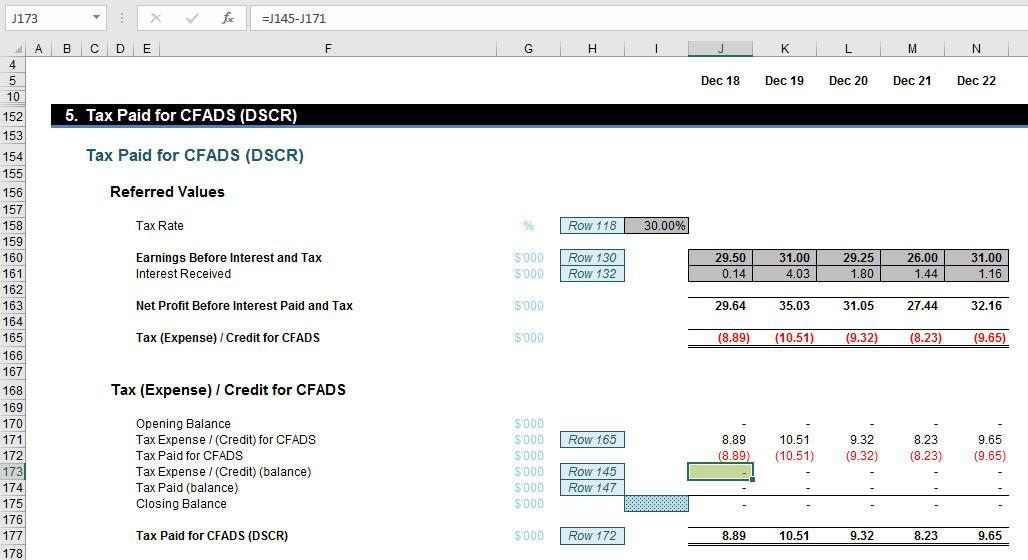
In this section, I have excluded Interest Paid.  This is not cheating.  CFADS is the Cash Flow Available for Debt Servicing so it is before Interest Paid.  Including Interest Paid would be wrong: this is a common mistake financial modellers make.

However, even though some modellers avoid this mistake they then forget to consider Interest Paid for the next period.  This is what row 173 considers it adds in the balancing figure after Tax Paid for CFADS has been determined.  The formula

adds back any missing amounts.  If this is not done, tax losses may affect timing of any Tax Paid for CFADS incorrectly.

Did you notice the heading of this section?  This calculation is for DSCR computations only.  I need to vary this for other sculpting procedures – but more on that later.

I am now able to construct CFADS:

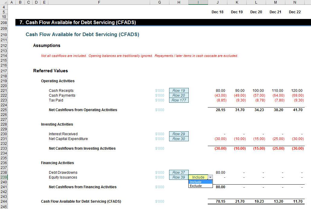
Do note that Tax Paid in row 223 of my example actually refers to the pre-Interest Paid tax figures.  Further, although equity cashflows are generally ignored, in some instances equity issuances will be included depending upon what capital raised may be used for and when the monies were received.  Finally, you should also realise that CFADS is generally accepted to be the cash for the period in question rather than the cumulative balance.

With no potential circular references and CFADS now evaluated, debt repayments and the corresponding interest can now be determined.  There are several ways this profile may be calculated (“sculpted”).  Let me look at three common ways in turn.

(1) Debt Service Coverage Ratio (DSCR) Approach

DSCR is a ratio frequently used by lenders to identify how “at risk” repayments of debt and payments of interest charges and fees (debt servicing) appear to be, using the ratio

These should all be cash flow figures.  Modellers often use P&L proxies, but this may lead to incorrect conclusions about the viability of a loan and more importantly, the business in general.

In our attached Excel file, with CFADS calculated, a target DSCR may be input which will identify the debt servicing required.  With Interest Paid based upon the Opening Debt Balance, Principal Paid is simply

Obviously, this will be subject to restrictions, such as the cash available and how much debt is left to be paid – but it’s all just mathematics!  Firstly, simply bring in all that you need:

Once Assumptions and Referred Values have been brought in, the calculations are straightforward:

In my example, the Target Debt Service is calculated in row 279, broken down into its constituent components, Interest Paid and Principal Paid in rows 297 and 312 respectively.

(2) Project Life Coverage Ratio (PLCR) Approach

One of the criticisms aimed at the DSCR method is that it does not take into account the time value of money.  PLCR rectifies this as it compares the present value of all future cash available and compares it to the current debt balance, viz.

Net Present Value is the free cash flows of CFADS so excludes any costs associated with debt – in particular Interest Paid.  Do remember the tax shield on interest paid: this needs to be excluded too.  For purposes of the principle of symmetrical returns (an underlying axiom of Net Present Value) – and also to avoid a circularity – Interest Received is also excluded.  Therefore, this gives rise to a revised Tax Paid calculation:

In my example, I assume the project life ends in the final period of the model.  To calculate closing debt balances, I know the closing debt balance is the opening balance of the next period, so my Target Closing Balance for any given period will be given by

The movement in the Target Closing Debt Balance will derive my Principal and Interest Paid can be deduced from the movement in the Opening Debt balance each period.  Using the attached Excel file:  

It should be noted that the appropriate interest rate to use here should be the post-tax cost of debt (i.e. the interest rate after tax).  The calculations are then relatively straightforward:

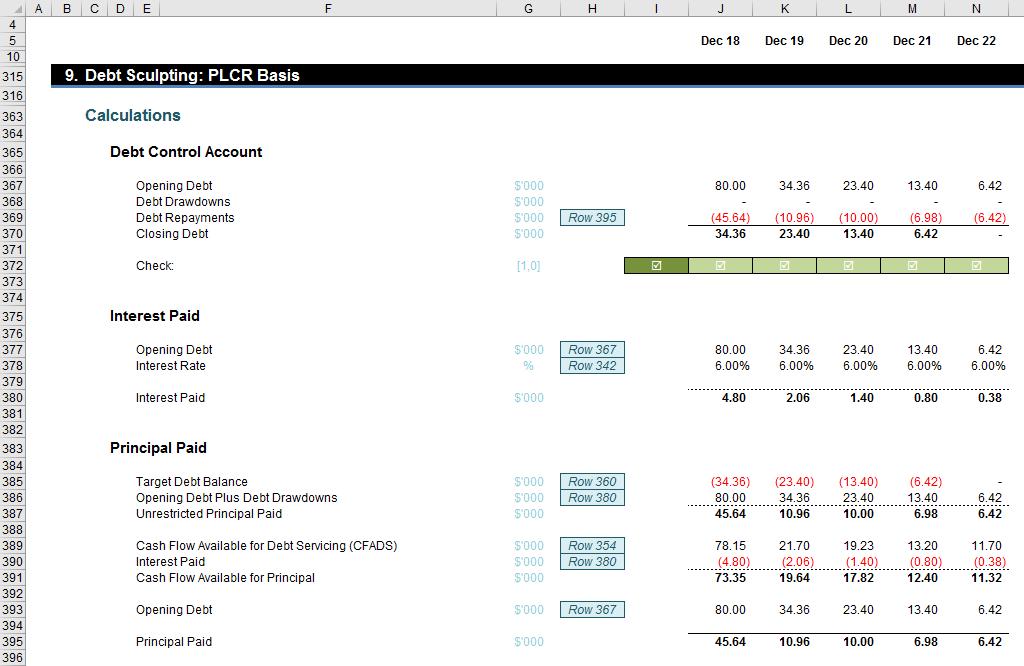
No circular and hence no macro are required.

(3) Loan Life Coverage Ratio (LLCR) Approach

The LLCR is essentially a restricted form of the PLCR method.  The sole difference is that instead of considering all future periods’ CFADS only available cashflows during the debt period are permissible for the NPV calculation. 

LLCR = NPV of Future CFADS Restricted to Debt Period / Opening Debt Balance

This methodology also uses the alternative Tax Paid calculations.  Again, the Principal and Interest Paid can be deduced from the movement in the Opening Debt balance each period:

These then lead to the calculations:

Putting it Altogether

In my example, I have created the three approaches, but now I need to add the relevant items back into my original Cash Flow Statement.  To do this, I will create a summary first:

This then feeds back into the Cash Flow Statement so that all rows now contain data:

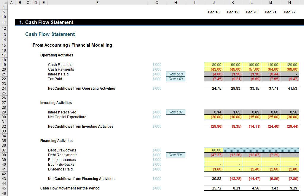
Even with these entries entered, there are no circularities; congratulations – you have created your very first debt sculptures using DSCR, PLCR and LLCR!

Word to the Wise

It is fair to say others have already provided examples of how to sculpt debt using formulae only.  The problem I have with most of these articles written is that they show you how to solve the problem with CFADS already given – but calculating CFADS is part of the problem.  I wanted to explicitly show you how to create CFADS in such a way it causes no such issues.

Regarding all three approaches, I have deliberately allowed drawdowns and repayments to occur in the same period.  This is unusual.  My rationale here really is that I must generate an Opening Debt Balance somehow (given no Balance Sheet) and I did not want to have too many periods in my model.

Please note that the attached Excel file allows you to switch between the three sculpting methods.  Whilst this technique is versatile and allows end users to switch as they see fit, it should be noted that the summary numbers may change depending upon the approach selected in cell H490.  This is because certain formulae depend upon values in earlier periods which are only calculated throughout the entire spreadsheet when this approach has actually been chosen.

Real-life modelling may add further complications such as two or more loans, stub periods, hybrid financing, interest during construction and interest calculated on average balances.  None of these problems are insurmountable.  Should you have a problem, feel free to drop me a line at liam.bastick@sumproduct.com.