Data Tables Re-Revisited: Care with Inputs

And so, I return yet again to a popular Excel feature: Data Tables.  To recap, Data Tables are ideal for executive summaries where you wish to show how changes in a particular input affect a key output.  However, as always with modelling, Keep It Simple Stupid (KISS).  If you can achieve the same functionality without using Data Tables in a simple, straightforward fashion, then do it that way.  

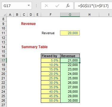
In this illustration, the key output revenue has been given in cell G11.  We want to summarise what happens if we increase (“flex”) this figure by a given percentage, with the inputs specified in cells F17:F26.  This can be simply computed by using the formula

in cell G17 and simply copying this calculation down. 

Data Tables should really be used when such simple calculations are not possible, and you want to flex one variable (known as a “one-variable” or “one-dimensional (1-D)” Data Table) or two (known as a “two-variable” or “two-dimensional (2-D)” Data Table).

You can create 1-dimensional versions (where the inputs go down a column or across a row) or 2-dimensional (where the inputs go both ways).  If you want to find out more about Data Tables in general, I would suggest referring to this article here.

Simple Example

From the attached Excel file, consider the following example:

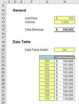
Here, like the last example, this illustration does not really warrant a Data Table, but I will put one in regardless.  All cells in yellow are inputs.  The calculation in cell H15 is extremely complex - =H12*H13!  But that’s not the point. 

Cell H20 contains >Data Validation, which generates a drop-down list of “On” or “Off” to choose from.  Cell H22 then contains a formula believe it or not:

i.e. the formula refers to the Total Revenue in cell H15 if the value in cell H20 is “On”.  The reason this cell appears to be a heading that says “Total Revenue” as well is due to custom number formatting.  That is, if we click on the cell, right-click and choose ‘Format Cells…’ (CTRL + 1), we can see the following formatting:

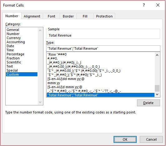
The ‘Number’ formatting is ‘Custom’ and has the key

This means that if the value is a non-negative number (i.e. zero or a positive number), the value will appear as “Total Revenue” (the text before the delimiting semi-colon), and if it is negative it will also appear as “Total Revenue” (the text after the semi-colon).  The reason this must be entered twice is otherwise if the number were negative text would appear as

i.e. with a minus sign in front of the text.  Just a little trick, that’s all.

After the required input values (100 to 110 inclusive, as displayed) have been hard coded into cells G23:G33, the range G22:H33 has been selected, and then a Data Table has been created by selecting ‘Data Table…’ from the ‘What-If Analysis’ drop-down in the ‘Forecast’ group of the ‘Data’ tab of the Ribbon, viz.

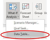
Since the inputs go down a column and the input cell is in cell H12, the resulting ‘Data Table’ dialog has been populated thus:

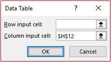
Assuming workbook calculations are set to ‘Automatic (ALT + T + O), that’s all you have to do – simple!

So, what’s the problem?

One of the things we always emphasise here at SumProduct (please link to ) is that models should be Consistent, Robust, Flexible and Transparent – something we call >CRaFT.  “Flexible” means the model should not contain superfluous hard code and should use consistent formulae wherever possible.  And therein lies the problem.  Let me explain.  Consider this revised example:

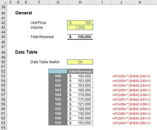
Here, the columnar inputs (cells G53:G63) have been replaced by a formula:

This seems to be fairly innocuous and theoretically, should make the worksheet more efficient as inputs do not need to be typed in twice.  However, look closer.  The values in cells H55:H63 are wrong.  This is a common trap.  It’s dangerous using formulaic inputs in a Data Table.

So what went wrong?

A 1-dimensional columnar Data Table works procedurally as follows:

1. Take the first input and put it in the input cell (so here, the value in cell G53 – 100 presently – would be copied as a value into cell H42)
2. This would cause the values in the formulaic inputs to update (so cells G53:G63 would be updated to [still] display 100, 101, …, 109, 110)
3. The result (cell H45, $100,000) would be recorded in the first row of outputs (cell H53)
4. The second input – currently 101 (cell G54) – would then be pasted as a value into the input cell (cell H42)
5. This would cause the values in the formulaic inputs to update (so cells G53:G63 would be updated to now display 101, 102, …, 110, 111 – these values have changed)
6. The result (cell H45, $101,000) would be recorded in the second row of outputs (cell H54) (this is why this output remains correct)
7. The third input – now revised to 103, not 102 (cell G55) – would then be pasted as a value into the input cell (cell H42)
8. This would cause the values in the formulaic inputs to update (so cells G53:G63 would be updated to now display 103, 104, …, 112, 113 – these values have changed)
9. The result (cell H45, $103,000, being $103 multiplied by 1,000) would be recorded in the third row of outputs (cell H55) (this is why this output is incorrect)
10. The fourth input – now revised to 106, not 103 (cell G56) – would then be pasted as a value into the input cell (cell H42)
11. This would cause the values in the formulaic inputs to update (so cells G53:G63 would be updated to now display 106, 107, …, 115, 116 – these values have changed)
12. The result (cell H45, $106,000, being $106 multiplied by 1,000) would be recorded in the fourth row of outputs (cell H56) (this is why this output is also incorrect)
13. And so on…
14. When all outputs have been determined, the Data Table input values (cells G53:G63) are then reset to the original values (100 to 110 inclusive).

Explained like this, it’s easy to see the problem.  If cell G53 had been left as a hard-coded value, or linked to an independent cell elsewhere, this would not have happened.  However, people don’t get this, and the internet is littered with end users moaning that their Data Tables are wrong and Excel makes errors.  It doesn’t; people do.  Be careful; use inputs!