
Calculating Depreciation for Existing Capital Expenditure
I was in two minds about writing this article (as opposed to my usual articles where I am out of my mind when I write them). This is not the sexiest topic I will ever cover. However, it is an area of financial modelling riddled with material significant errors. Sorry, dear reader, but it needs to be addressed.
Few would quibble that:
- Capital expenditure tends to be a major area of expenditure for a business
- Existing fixed (non-current) assets typically represent a significant amount on the Balance Sheet at any given time
- Income Statements are scrutinised by many stakeholders and need to be as accurate as possible.
Therefore, calculating the correct depreciation for existing non-current assets is a very big deal. As a model auditor for nearly 30 years, I have to frighten you and tell you that 99%+ of all forecast models get this figure wrong.
Let me explain. Imagine you had a classification of fixed assets on your Opening Balance Sheet (say “Vehicles”) with a cited remaining (average) useful economic life of four years. Assuming your company amortises on a straight-line basis and that the assets have no residual value, you would therefore depreciate these assets by $25m for each of the next four years, correct?
I hate to be the bearer of bad news, but that’s wrong.
Even if you spent the same amount each year on capital expenditure, it would be wrong. This is because we are only considering existing capital expenditure: new capital expenditure is calculated separately – we simply need to wind down the existing amount.
Further, assuming assets are depreciated as they are added, the economic life must be FIVE years not four (since the final depreciation calculations started last year, as there will be no additions to existing capital expenditure this year by definition).
If I assume the business started 10 years ago, the capital expenditure must be the following:

To generate a steady state of $100m with the same capital expenditure each period and four years of depreciation left, I must be acquiring assets each year of $50m with a five-year useful economic life. It’s easier to understand when shown like this – but it’s not obvious.
Since assets “roll off” each year, the depreciation is not 25% straight line each year: it’s 40%, 30%, 20% and 10% for the next four years respectively of the current $100m. I am betting no one reading this is presently modelling it this way. If you are, feel smug and feel free to email someonewhocares@aicpa.com. Your email might bounce.
The problem is, I have simplified the issue above. Capital expenditure may vary each year. You may also be modelling sub-annually (e.g. monthly or annually) where capital expenditure is seasonal too. It’s going to get more complicated.
How can we model this with a reasonable amount of accuracy? Let me try to keep the solution from becoming too unwieldly, by implementing the following assumptions:
- I will assume we are modelling quarterly (it generates fewer periods to consider than monthly, but addresses similar issues)
- I will assume that the proportions of expenditure each year are the same for each corresponding quarter
- I will assume a constant growth rate in past capital expenditure (you could estimate this by Compound Annual Growth Rates in practice).
These assumptions are not unreasonable when you consider that normally we have no better information to go on.
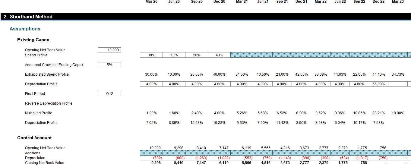
I will use the following attached Excel file to assist me. The trick here is that the number of periods must be at least double the economic life assumed. The reason for this will become clear shortly.
I will work with the following assumptions:
It should be noted that:
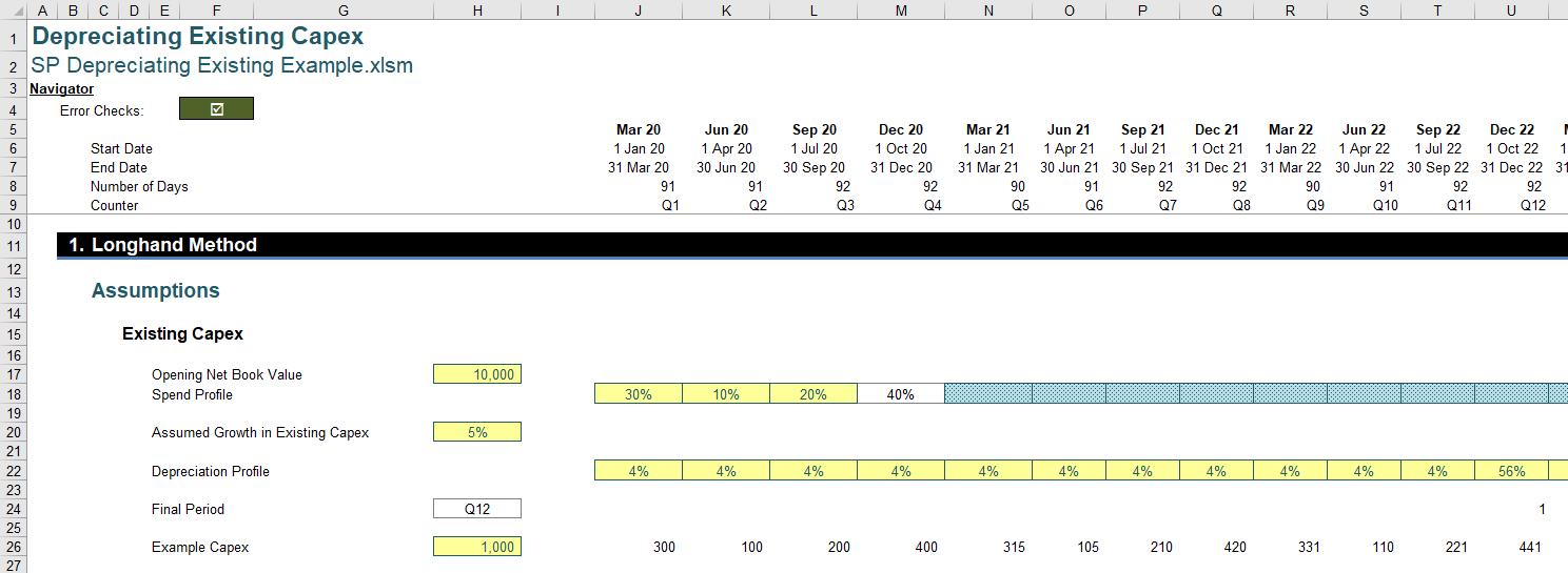
- This model is calculated quarterly
- I assume you are comfortable with the dates and counter (rows 5:9 inclusive)
- Cell H18 represents the Opening Net Book Value (NBV) as at the Balance Sheet date. Here, I have assumed an amount of $10,000
- Row 19 provides the profile for expenditure incurred each quarter (as a percentage). It is only shown for the first four quarters, as it is assumed this profile recurs for all subsequent periods. The formula in cell M18 (=1-SUM(J18:L18)) simply ensures the percentages add up to 100% for each calendar year
- Cell H20 assumes that capital expenditure has been grown exponentially at a constant rate. If you don’t like this simplifying assumption, I suggest you write your own article and submit for a PhD in Mathematics
- Row 22 (the Depreciation Profile) could be any sequence of percentages as long as they add up to precisely 100% (my spreadsheet ensures this with a formula in the final year to make up any difference)
- The formula in cells J24:AW24 flags the first period where the percentages add to exactly 100%:
- =(SUM($J22:J22)=1)*(SUM($I24:I24)=0)
- This places a ‘1’ in the final period so that it may be readily identified (in cell U24 in the above screenshot)
- Cell H24 identifies the Final Period for the purposes of the ensuing calculations. This may be different to the period identified in cells J24:AW24. This is a subtle point. As the intention is to look for a cyclical pattern, we will be focusing on calendar years. Therefore, if the economic life is not a whole number of years, the number is rounded up to the next integer. This requires rounding the period up to the nearest multiple of four (4) – the number of quarters in a year. The MROUND function serves this purpose, and SUMIF is used to identify where the ‘1’ is as this value can appear once and only once:
=MROUND(SUMIF(J24:AW24,1,J9:AW9),Quarters_in_Year) - =MROUND(SUMIF(J24:AW24,1,J9:AW9),Quarters_in_Year)
- The final row shown, row 26, simply depicts how a starting capital expenditure amount of $1,000 would be split over the fist four quarters and then consequently grown thereafter:
- =IF(J$9<=Quarters_in_Year,J$18*$H26,F26*(1+$H$20)).
The aim is to create a depreciation grid out of this capital expenditure profile, using the depreciation rates input too. I have covered this in a previous article when I explained how the OFFSET function could be used to calculate depreciation. As a recap…
Aside: OFFSET
The OFFSET function, which employs the following syntax:
OFFSET(Reference, Rows, Columns, [Height], [Width])
The arguments in square brackets (Height and Width) can be omitted from the formula – but they will prove to be useful here.
OFFSET(Reference, Rows, Columns) will select a reference Rows rows down (-Rows would be Rows rows up) and Columns columns to the right (-Columns would be Columns columns to the left) of the Reference. For example, consider the following grid:
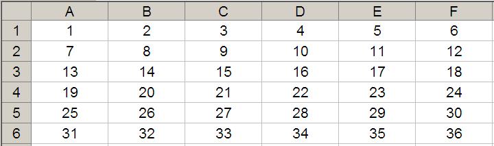
OFFSET(A1,2,3) would take us two rows down and three columns across to cell D3. Therefore, OFFSET(A1,2,3) = 16, viz.
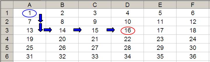
OFFSET(D4,-1,-2) would take us one row up and two columns to the left to cell B3. Therefore, OFFSET(D4,-1,-2) = 14, viz.
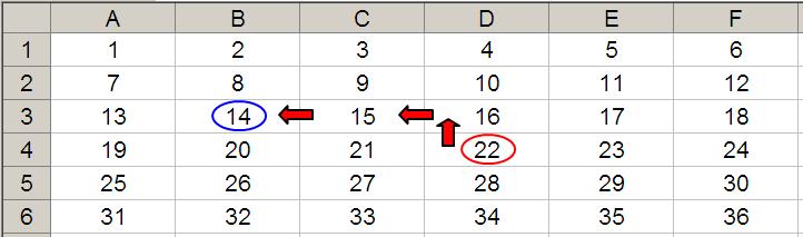
Let me extend the formula to OFFSET(D4,-1,-2,-2,3). It would again take us to cell B3 but then we would select a range based on the Height and Width parameters. The Height would be two rows going up the sheet, with row 3 as the base (i.e. rows 2 and 3), and the Width would be three columns going from left to right, with column B as the base (i.e. columns B, C and D).
Hence OFFSET(D4,-1,-2,-2,3) would select the range B2:D3, viz.
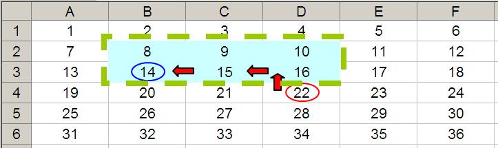
Note that OFFSET(D4,-1,-2,-2,3) = #VALUE! since Excel cannot display a matrix in one cell, but it does recognise it. However, if after typing in OFFSET(D4,-1,-2,-2,3) we press CTRL + SHIFT + ENTER, we turn the formula into an array formula: {OFFSET(D4,-1,-2,-2,3)} (do not type the braces in, they will appear automatically as part of the Excel syntax). This gives a value of 8, which is the value in the top left-hand corner of the matrix, but Excel is storing more than just that. This can be seen as follows:
- SUM(OFFSET(D4,-1,-2,-2,3)) = 72 (i.e. SUM(B2:D3))
- AVERAGE(OFFSET(D4,-1,-2,-2,3)) = 12 (i.e. AVERAGE(B2:D3)).
I will use OFFSET and SUM(OFFSET) to assist me here.
Returning to Our Problem
I can build a depreciation grid using OFFSET:
The formulae in column H transpose the capital expenditure:
=OFFSET($I$26,,ROWS($E$33:$E33))
This formula starts in cell I26 and moves across one column for each row the formula is copied down. It’s a great common use of the OFFSET function.
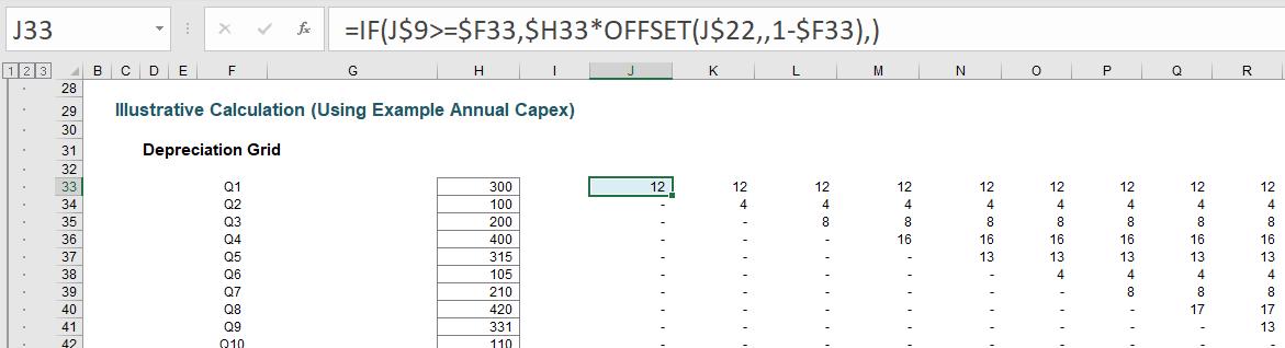
The formula in the grid,
=IF(J$9>=$F33,$H33*OFFSET(J$22,,1-$F33),)
only calculates once the capital expenditure has been incurred (hence the condition J$9>=$F33, i.e. the quarter must be greater than or equal to the quarter the capex occurred). The OFFSET formula is used to ensure the correct percentages are used in each period (so that the percentages move across one period each quarter).
With an assumption of an economic life of three (3) years or 12 quarters, the depreciation has “matured”: depreciation as a proportion of the opening NBV repeats a cycle on annual basis, viz.
Although it has now reached a steady state, I cannot use these percentages as this assumes additions continue to be included. However, I can consider the following numbers from the depreciation grid:
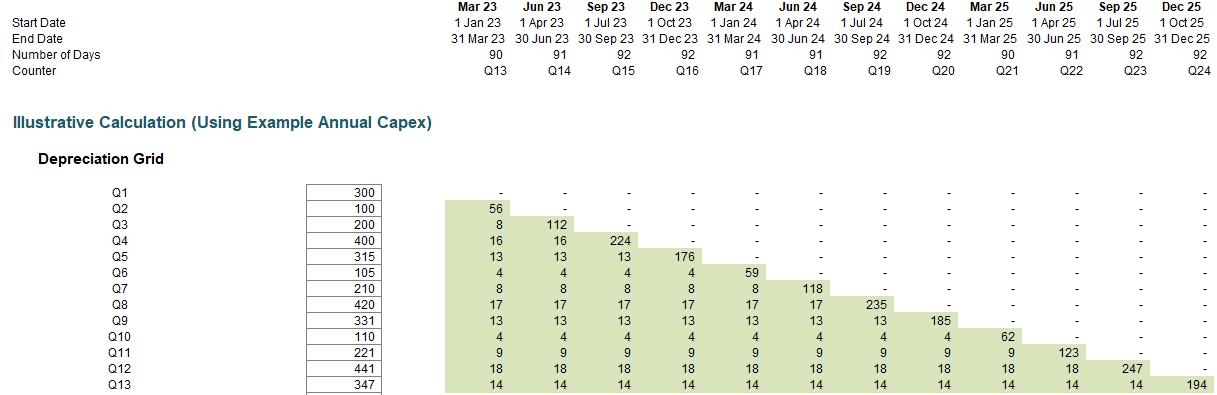
Whilst the cycle repeats from Q12, I must start with Q13. This is because Q13 aligns with Q1, Q14 aligns with Q2, etc. This is why the model needs to have a time horizon of at least twice the economic life assumed.
Obviously, these numbers are irrelevant for my opening NBV ($10,000), but I can pro-rate. If I sum all of the shaded values in the Q13 column and calculate it as a proportion of the total shaded sum (the total depreciation for expenditure incurred in Q2 to Q13 for Q13 to Q24), I will have my relevant depreciation percentage. Calculating this percentage and multiplying it by $10,000 will give me my depreciation for Q1.
Similarly, summing all of the values in the Q14 column and dividing that by the total value of the shaded area will provide me with my depreciation percentage for Q2. The formulae may not be the simplest, but the concept is fairly straightforward.
Allowing for the economic life to change the formula for Q1 is given by
=SUM(OFFSET(J$33,1,$H$24,$H24,))/SUM(OFFSET($I$33,1,$H$24+1,$H$24,$H$24))
The numerator of this quotient calculates the total in the first shaded column and the denominator computes the total shaded amount:
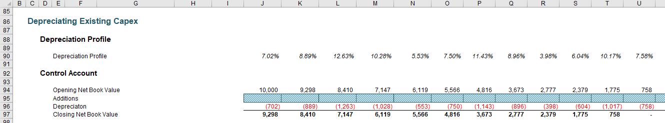
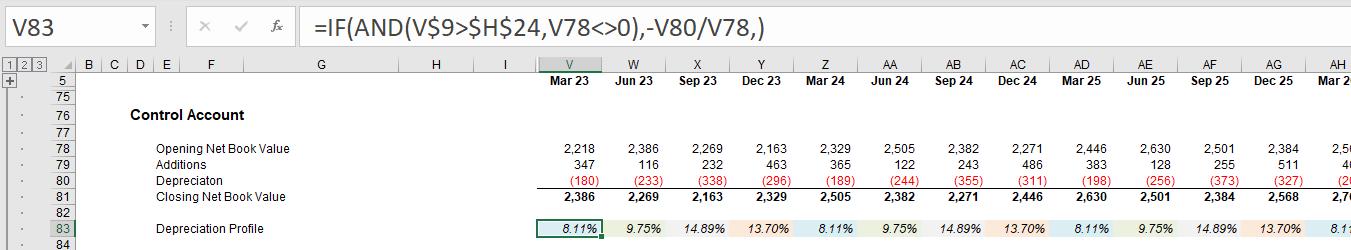
There you have it: I can use these percentages to amortise my opening NBV using the above control account. It’s not perfect, but a better approximation than simple straight-line depreciation. This can be important for getting P&L multiples and tax calculations correct.
For the record, my attached Excel file shows an alternative computation that does not require a depreciation grid:
Conscious I have probably put you through enough for one article, I won’t go through all of the technical aspects here – suffice to say you can copy this calculation into your own spreadsheets as required.
Word to the Wise
This is an area of financial modelling even advanced modellers and accountants get wrong – on a fundamental basis. I do not claim my approach is perfect (it isn’t), but it provides a better approximation for estimating the depreciation profile of existing capital expenditure – which is important when the numbers are material.
I promise we’ll do something simpler next time out, like considering the impact of tensor analysis in relation to the Theory of General Relativity…