
Avoiding Bad Hyperlinks
Liam Bastick, director (and Excel MVP) with SumProduct Pty Ltd, highlights some of the common issues and scenarios in financial modelling / Excel spreadsheeting. This article looks at a simple way of avoiding a very common issue with hyperlinks.
Hyperlink Tips
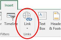
In Excel, hyperlinks are fairly straightforward to use and readily accessed via one of two keyboard shortcuts, either ALT + I + I or CTRL + K. Alternatively, it can be inserted from the ‘Links’ grouping on the ‘Insert’ tab of the Ribbon:
Hyperlinks can be used to link to a variety of places, but in this instance, I will focus on linking to elsewhere within the same work.
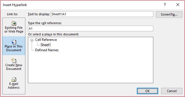
To create a hyperlink, first select the cell or range of cells that you wish to act as the hyperlink (i.e. clicking on any of these cells will activate the hyperlink). Then, open the ‘Insert Hyperlink’ dialog box (above) and select ‘Place in This Document’ as the ‘Link to:’, which will change the appearance of the rest of the dialog box.
Insert the text for the hyperlink in the ‘Text to display:’ input box (clicking on the ‘ScreenTip…’ macro button will allow you to create an informative message in a message box when you hover over the hyperlink).
The next two input boxes, ‘Type the cell reference:’ and ‘Or select a place in this document:’, work in tandem – sort of:
- If you type a cell reference in the first input box without making a selection in the second input box, the hyperlink will link to the cell reference on the current (active) worksheet; or
- If you type a cell reference in the first input box and select a worksheet reference in the second box, the hyperlink will link to the specified cell in the given worksheet. In my example above, this hyperlink will jump to Sheet1!A1.
Where you require linking to a specific cell, obviously link to that cell; however, if you are ‘generally’ linking to a spreadsheet, consider linking to the CTRL + HOME cell. To maintain a ‘professional’ feel to your spreadsheets, consider linking so that the sheet ‘resets’ to the top left-hand corner, regardless of where it was last viewed. The cell that will do this is known as the home cell. This cell can be readily identified. If there is a split or frozen pane on the worksheet, then cell A1 will not be the correct cell. The cell can be identified by the keyboard shortcut CTRL + HOME. It is always the top left-hand corner of the bottom right hand quadrant of any frozen panes. It is the top left-hand corner cell of the range selected to freeze panes in the first place, viz.

A better tip is not to link using a worksheet name and cell reference. There’s a very simple reason for this. If the destination worksheet’s name is changed, clicking on the hyperlink will produce the following dialog box:
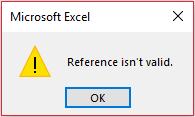
Unlike formulae, if a worksheet name is changed, the reference will not update automatically (in fact if rows / columns are inserted / deleted, the cell reference will not move either). Therefore, always give the destination cell for your hyperlink a range name.
To do this, simply select the cell you wish to link to and either right click to get ‘Define Name…’ on the shortcut menu or else use the keyboard shortcut ALT + M + M + D. Then, if you create the hyperlink as before, this time select a ‘Defined Name’ (i.e. a pre-defined range name) in the second input box, this will link to the cell(s) specified:
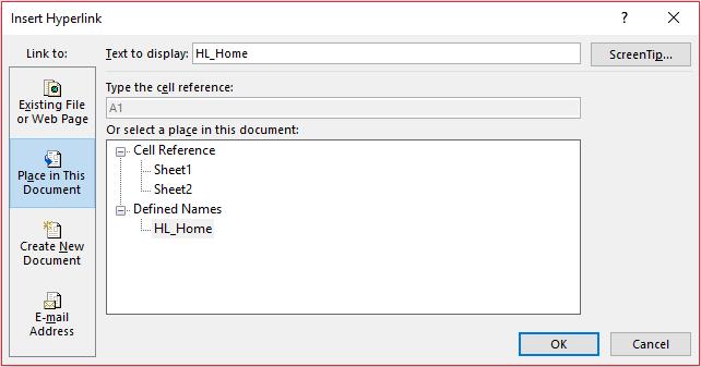
This is the recommended option, where available, if you wish to link to cell(s) on another worksheet within the same workbook. This is because if the destination worksheet’s sheet name were to be changed, the link would still work. Note also that my range name starts with “HL_” – this prefix methodology (HL for hyperlink) is a good way to find all your hyperlink destination range names if you have many range names to sift through.
It is recommended that range names are used for the destination so that the hyperlink will work if the worksheet name to which the link points is changed.
When creating a number of hyperlinks simultaneously, the function:
=HYPERLINK(link_location,[friendly_name])
may be used instead. The link_location is as before (and can be a range name), whereas the optional argument friendly_name will be the text displayed in the hyperlink. Do note screen tips cannot be created using the HYPERLINK function.
Word to the Wise
The HYPERLINK function does not require the use of range names, but the syntax and formatting can be much more complex if range names are not used.
Not all functions will work with HYPERLINK. It is not always clear why this may be. It is best trying to use HYPERLINK on a trial and error basis. However, it should be borne in mind that if the hyperlink reference is static, the Insert Hyperlink technique, described in detail above, may be the better alternative.
If you have a query for the Thought section, please feel free to drop Liam a line at liam.bastick@sumproduct.com or visit the SumProduct website.