
Aggregating Aggravating Time Periods
If you have ever built a financial model, you will have come to realise that recipients always want greater detail in the earlier periods and are then happy to have summaries for later dates. For example, in a budget model it is not unusual for the first 12 months to be reported monthly, then the next two years quarterly, with annual summaries thereafter.
However, that’s not how you should model. That’s how you should report.
There are lots of texts out there advocating what is and what isn’t Best Practice when it comes to building a financial model. At SumProduct, we push CRaFT:

Here, I want to emphasis consistency. In particular, all modelling should be undertaken at the same level of granularity, then summarised as required in the output sheets. Therefore, for my example above, I would model monthly and then summarise the quarterly and annual periods later with either the LOOKUP or SUMIF functions.
Let me explain with a comprehensive example from the attached Excel file. Consider the following monthly data:
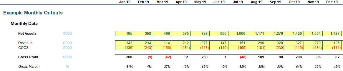
The model has five years’ (60 months’) data; only some is reproduced (above) here. In this instance, I want to report the first calendar year monthly, the next year quarterly, the next year half-yearly and the remainder annually. Therefore, I built a generic interface that will provide lots of variation, assuming as time moves on, granularity will be similar or else become more and more high level:
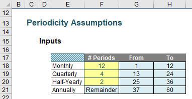
The assumptions are entered in the yellow cells, cells F18:F20, with the remainder of the months reported on an annual basis. Each period has been provided a period number, with the range of period numbers named LU_Number_of_Periods (“LU” refers to “Look Up”). This means that the total number of periods (60) is given by MAX(LU_Number_of_Periods).
The yellow cells used a data validation list (ALT + D + L), where the only values allowed are “None”, 1, 2, 3, …, 59 and 60 (the maximum period number). This helps keep the formulae in cells G18:H21 manageable.
Cell G18 (Monthly From period number) is reasonably straightforward:
=IF(OR($F18="None",$F18=""),"None",1)
Essentially, the start period is 1 unless the Monthly input cell is blank or has had “None” selected. Similarly, cell H18 (Monthly To end period) is not too complex:
=IF(OR($F18="None",$F18=""),"None",MIN($F18,MAX(LU_Number_of_Periods)))
Again, this checks that there is a number in cell F18, and then ensures the final period cannot be greater than the maximum period number (in case data validation is not updated when the model is edited).
The next three rows are fairly similar, so I will only consider row 19. Cell G19 (Quarterly From period number) contains the formula
=IF(OR($F19="None",$F19="",MAX($H$18:$H18)=MAX(LU_Number_of_Periods)),"None",MAX($H$18:$H18)+1)
This formula adds one to the Monthly To period number (cell H18) provided this makes sense. The MAX function is used so that if cell H18 is “None” (i.e. there are no monthly reporting periods), MAX(“None”)+1 gives a value of 1 rather than “None”+1 which gives the error #VALUE!
Cell H19 (Quarterly To period number) contains a slightly longer formula:
=IF(OR($F19="None",$F19="",$H18=MAX(LU_Number_of_Periods)),"None",MIN($F19*Months_in_Quarter+$G19-1,MAX(LU_Number_of_Periods)))
It takes the Quarterly From period number and calculates what the end period number is subject to it not exceeding the maximum number of periods. The formulae in the two rows below use similar calculations, but exchange Months_in_Quarter for Months_in_Half_Yr and Months_in_Year instead.
Now it’s not all about consistency. Another key quality is transparency, and by that, I mean you can follow it on a piece of paper (if printed out) without having to refer to the formula bar in Excel. Sorry for the tiny graphic, but it gives an idea of how the presentation works:
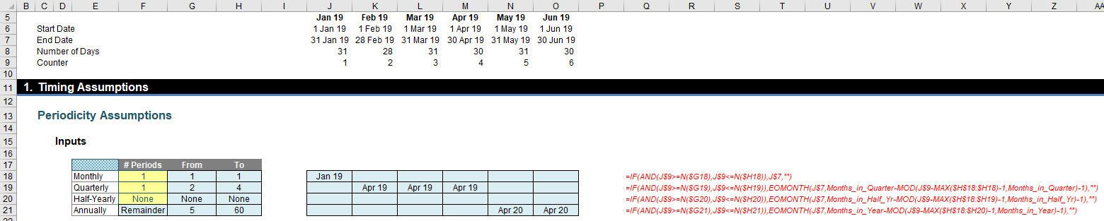
The idea is that the dates displayed in cells J18:O21 (pictured) show the period end that the periods are included in (e.g. Mar 19 is included in the Apr 19 quarter and Jun 19 is included in the Apr 20 year). The formulae aren’t particularly, er, nice. Cell J18 contains the formula
=IF(AND(J$9>=N($G18),J$9<=N($H18)),J$7,"")
which presents the month end of the period if it is one of the periods that is reported monthly. However, the formula in cell J19 is slightly more sophisticated:
=IF(AND(J$9>=N($G19),J$9<=N($H19)),EOMONTH(J$7,Months_in_Quarter-MOD(J$9-MAX($H$18:$H18)-1,Months_in_Quarter)-1),"")
Not quite as straightforward? That’s because I need EOMONTH(Date,Number_of_Periods) to calculate the end of the month Number_of_Periods from now and this second argument uses the MOD function (Months_in_Quarter-MOD(J$9-MAX($H$18:$H18)-1,Months_in_Quarter)-1) to work out how many months to go forward. For example:
- If I am in the first period of the quarter, I need to calculate the end of the month two months from now
- If I am in the second period of the quarter, I need to calculate the end of the following month
- If I am in the final period of the quarter, I need to calculate the end of the month.
Similar formulae are required for the half-yearly and annual computations too. Once you have these dates, the next set of calculations are much simpler:
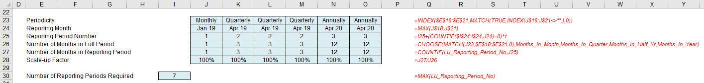
The formula in J23 (Periodicity),
=INDEX($E$18:$E$21,MATCH(TRUE,INDEX(J$18:J$21<>"",),0))
utilises a technique observant readers will note I use time and time again. This finds the first non-empty cell in the range J$18:J$21 and returns the corresponding label in cells $E$18:$E$21 (namely “Monthly”, “Quarterly”, “Half-Yearly” or “Annually”). This is useful for determining how many months there should be in the corresponding reporting period (e.g. 1 for “Monthly”, 3 for “Quarterly” and so on).
Cell J24 (Reporting Month) locates the date in the corresponding column in rows 18:21, viz.
=MAX(J$18:J$21)
That’s fairly straightforward. The next formula, in cell J25 (Reporting Period Number) is a little more elaborate:
=I25+(COUNTIF($I$24:I$24,J24)=0)*1
This adds one to the cell immediately to the left if the date in row 24 is different from all earlier periods’ dates. This provides all the reporting periods and the largest value represents the total (maximum) number of output reporting periods required. Given the range of values in row 25 is called LU_Reporting_Period_No, cell I30 therefore calculates this number:
=MAX(LU_Reporting_Period_No)
Returning to the main array of formulae, cell J26 (Number of Months in Full Period) calculates the number of months in a full reporting period using the CHOOSE function:
=CHOOSE(MATCH(J23,$E$18:$E$21,0),Months_in_Month,Months_in_Quarter,Months_in_Half_Yr,Months_in_Year)
whereas the formula in cell J27 (Number of Months in Reporting Period) calculates the actual number of months in each period. This is because the final period may be incomplete and we may wish to gross up the final output period in order to compare like with like data. The formula in cell J27 is thus given by:
=COUNTIF(LU_Reporting_Period_No,J25)
Finally, cell J28 (Scale-up Factor) determines what proportion each actual reporting period is of its “full” reporting period:
=J27/J26.
That’s all we need to produce our reporting period outputs:
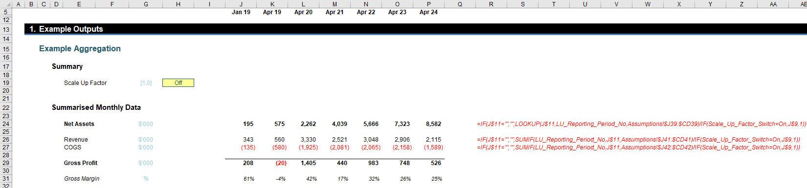
Before I explain these output formulae, it should be noted there are hidden rows (6:11):
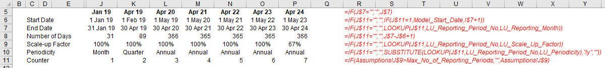
I am not going to go into all of these formulae, suffice to say that row 11 drives many of the other rows, based upon the calculations undertaken earlier.
Returning to our outputs, J24 refers to Net Assets which is a Balance Sheet item, so therefore we only require the final month’s value for the reporting period. This is achieved using the formula
=IF(J$11="","",LOOKUP(J$11,LU_Reporting_Period_No,Assumptions!$J39:$CD39)/IF(Scale_Up_Factor_Switch=On,J$9,1))
since LOOKUP seeks out the final period when dates are in ascending order (which they are). The check whether hidden cell J$11 is blank is to ensure the report is not continued for periods beyond which there is data.
The expression
IF(Scale_Up_Factor_Switch=On,J$9,1))
simply grosses up the value for any part-period reporting (assuming the switch in cell H19 is set to “On”). The formula for cell J26 (Revenue) sums all relevant periods instead:
=IF(J$11="","",SUMIF(LU_Reporting_Period_No,J$11,Assumptions!$J41:$CD41)/IF(Scale_Up_Factor_Switch=On,J$9,1))
hence the use of SUMIF rather than LOOKUP. The formula for COGS is similar and then the last two rows are simply calculations rather than more LOOKUP or SUMIF formulae.
Word to the Wise
This may seem like overkill, but this is a comprehensive example that can be slotted into existing models fairly easily. It is both consistent and transparent and allows you to model at the lowest level of granularity rather than attempt to derive formulae which work in different periods (an error made by even the most experienced modellers far too often, where they then realise they cannot reconcile amounts when data is aggregated in a different way).
Please use this technique (or one similar); don’t fall into the common modelling trap.