
What’s New in Excel 2019
22 November 2018
Last month we mentioned Office 2019 was now Commercially Available. We thought we’d better do some digging and see what was new (compared to Excel 2016, rather than Office 365). There really wasn’t any room in last month’s newsletter, so please forgive our tardiness. However, we aim to put it right now!
New Functions
Yes, we know we’ve done this before but for completeness, there are six new functions in Excel 2019 (compared to Excel 2016). These comprise:
- IFS
- SWITCH
- CONCAT
- TEXTJOIN
- MAXIFS
- MINIFS.
Let’s go through them.
IFS
As model developers and reviewers, we must confess we remain unconvinced about this one. If you have ever used a formula with nested IF statements, e.g.
=IF(IF(IF…
then maybe this function is for you – however, if you have ever written Excel formulae like this, then maybe Excel isn’t for you! There are usually better ways of writing the formula using CHOOSE or >INDEX(MATCH) for example.
The syntax is as follows:
IFS(logical_test1, value_if_true1, [logical_test2, value_if_true2], [logical_test3, value_if_true3],…)
where:
- logical_test1 is a logical condition that evaluates to TRUE or FALSE;
- value_if_true1 is the result to be returned if logical_test1 evaluates to TRUE. This may be empty
- logical_test2 (and onwards) are further conditions that evaluate to TRUE or FALSE also
- value_if_true2 (and onwards) are the respective results to be returned if the corresponding logical_test evaluates to TRUE. Any or all may be empty.
Since functions are limited to 254 arguments (sometimes known as parameters), the new IFS function can contain 127 pairs of conditions and results.
One thing to note is that IFS is not quite the same as IF. With the IF statement, the third argument corresponds to what do if the logical_test is not TRUE (i.e. it is an ELSE condition). IFS does not have an inherent ELSE condition, but it can be easily generated. All you have to do is make the final logical_test equal to a condition which is always trues such as TRUE or 1=1 (say).
Other issues to consider:
- Whilst the value_if_true may be empty, it must not be omitted. Having an odd number of arguments in an IFS statement would give rise to the “You’ve entered too few arguments for this function” error message.
- If a logical_test is not actually a logical test (e.g. it evaluates to something other than TRUE or FALSE, the function returns an #VALUE! error. Numbers still appear to work though: any number than zero evaluates as TRUE and zero is considered to be FALSE.
- If no TRUE conditions are found, this function returns the #N/A! error.
To show how it works, consider the following example.
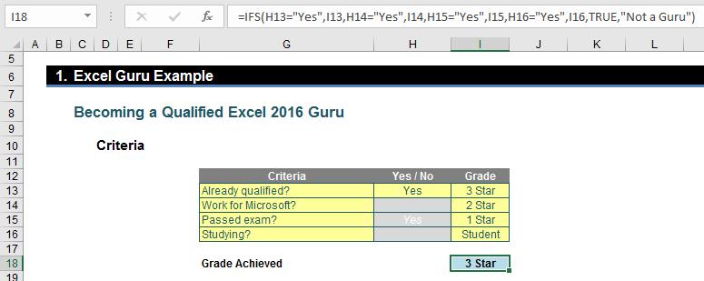
Here, would-be gurus are graded based on evaluation criteria in the table, applied in a particular order:
=IFS(H13="Yes",I13,H14="Yes",I14,H15="Yes",I15,H16="Yes",I16,TRUE,"Not a Guru")
I think it’s safe that although it is reasonably straightforward to follow, it is entirely reasonable to say it’s not the prettiest, most elegant formula ever put to Excel paper. In particular, do pay heed to the final logical_test: TRUE. This ensures we have an ELSE condition as discussed above.
To be fair, one similar solution using legacy Excel functions isn’t any better:
=IF(H13="Yes",I13,IF(H14="Yes",I14,IF(H15="Yes",I15,IF(H16="Yes",I16,"Not a Guru"))))
Lovely.
SWITCH
SWITCH is already available in many alternative programming languages and can simplify potentially horrible formulae. This function evaluates an expression against a list of values and returns the result corresponding to the first matching value. If there is no match, an optional default value may be returned. The syntax is as follows:
SWITCH(expression, value1, result1, [default or value2, result2],…[default or valueN, resultN])
where:
- expression is the value that will be compared against the values (value1 to valueN) cited
- value1 to valueN are the values that will be compared against the expression
- result1 to result are the values, references or formulae results to be returned when the corresponding valueN argument matches the expression. The result must be supplied for each corresponding valueN argument
- default is an optional value to return in case no matches are found in the valueN expressions. The default argument is identified by having no corresponding result expression, i.e. it must be the final argument in the function where the function contains an odd, rather than an even, number of arguments. If no default argument is supplied and no match is found this function returns the #N/A! error.
To illustrate, consider the following painful formula:
=SWITCH(MID($G13,SEARCH("-",$G13)+1,SEARCH("-",$G13,(SEARCH("-",$G13)+1))-SEARCH("-",$G13)-1),"XS","Extra Small","S","Small","M","Medium","L","Large","XL","Extra Large","Not Specified")
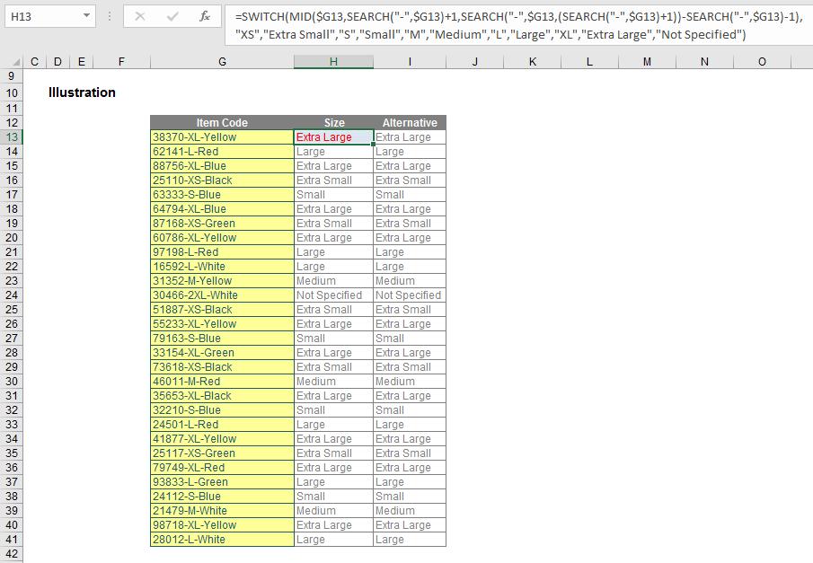
The expression here is
MID($G13,SEARCH("-",$G13)+1,SEARCH("-",$G13,(SEARCH("-",$G13)+1))-SEARCH("-",$G13)-1)
which is determining what is contained between the two hyphens (for more on text string functions, please see text messages). It is horrible, and that’s the point. The formula then considers what the values may be (“XL”,”M”) and what value should be returned as a consequence (“Extra Large”, “Medium”).
The corresponding Excel formula before SWITCH would have been a nightmare:
=IF(MID($G13,SEARCH("-",$G13)+1,SEARCH("-",$G13,(SEARCH("-",$G13)+1))-SEARCH("-",$G13)-1)="XS","Extra Small",
IF(MID($G13,SEARCH("-",$G13)+1,SEARCH("-",$G13,(SEARCH("-",$G13)+1))-SEARCH("-",$G13)-1)="S","Small",
IF(MID($G13,SEARCH("-",$G13)+1,SEARCH("-",$G13,(SEARCH("-",$G13)+1))-SEARCH("-",$G13)-1)="M","Medium",
IF(MID($G13,SEARCH("-",$G13)+1,SEARCH("-",$G13,(SEARCH("-",$G13)+1))-SEARCH("-",$G13)-1)="L","Large",
IF(MID($G13,SEARCH("-",$G13)+1,SEARCH("-",$G13,(SEARCH("-",$G13)+1))-SEARCH("-",$G13)-1)="XL","Extra Large","Not Specified")))))
CONCAT
This function replaces the CONCATENATE function. The CONCAT function combines the text from multiple ranges and / or text strings:
CONCAT(text1, [text2],…)
where:
- text1 is the text item to be joined
- text2 (onwards) are the additional items to be joined.
For example, consider the following illustration:
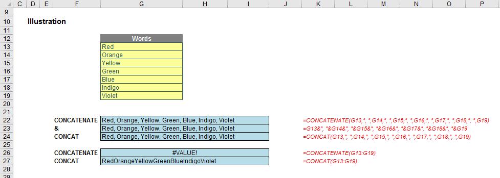
Upon first glance, CONCAT does the same thing as the legacy CONCATENATE function or & (ampersand) operator, but is just easier to spell. However, it is a little more than that: CONCATENATE will not cope with highlighting a contiguous range (it will just return the #VALUE! error); CONCAT will concatenate them all.
TEXTJOIN
The TEXTJOIN function combines the text from multiple ranges and / or text strings and includes a delimiter to be specified between each text value to be combined. If the delimiter is an empty text string, this function will effectively concatenate the ranges similarly to the CONCAT function. Its syntax is
TEXTJOIN(delimiter, ignore_empty, text1, [text2], …)
where:
- delimiter is a text string (which may be empty) with characters contained within inverted commas (double quotes). If a number is supplied, it will be treated as text
- ignore_empty ignores empty cells if TRUE or the argument is unspecified (i.e. is blank)
- text1 is a text item to be joined
- text2 (onwards) are additional items to be joined up to a maximum of 252 arguments. If the resulting string contains more than 32,767 characters TEXTJOIN returns the #VALUE! error.
TEXTJOIN is more powerful than CONCAT. To highlight this, consider the following examples:
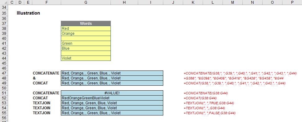
Here, in the formulae on rows 53 and 54, empty cells in a contiguous range may be ignored and delimiters only need to be specified once. When you compare to CONCAT, you do begin to wonder why you need it – perhaps to soften the demise of CONCATENATE..?
MAXIFS and MINIFS
The last two new functions I am going to combine – and not with TEXTJOIN!
MAXIFS(max_range, criterion_range1, criterion1, [criterion_range2, criterion2], ...)
returns the maximum value among cells specified by a given set of conditions or criteria, where:
- max_range is the actual range of cells in which the maximum is to be determined
- criterion_range1 is the set of cells to evaluate with the criterion specified
- criterion1 is the criterion in the form of a number, expression or text that defines which cells will be evaluated as a maximum
- criterion_range2 (onwards) and criterion2 (onwards) are the additional ranges and their associated criteria. 126 range / criterion pairs may be specified. All ranges must have the same dimensions otherwise the function returns an #VALUE! error.
MINIFS behaves similarly but returns the minimum rather than the maximum value among cells specified by a given set of conditions or criteria.
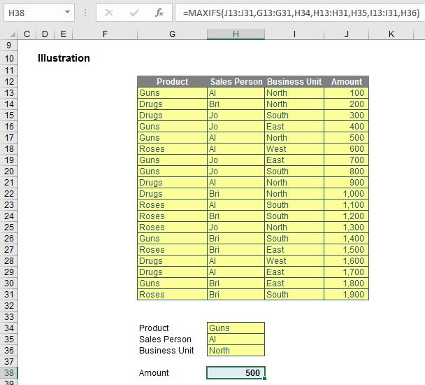
This example is preferable to its standard Excel counterpart:
{=MAX(IF(G13:G31=H34,IF(H13:H31=H35,IF(I13:I31=H36,J13:J31))))}
Array formulae are cumbersome and not readily understood.
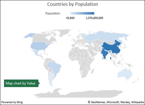
New Charts
You can create a map chart to compare values and show categories across geographical regions. This may be used when you have geographical regions in your data, like countries / regions, states, counties or postal codes.
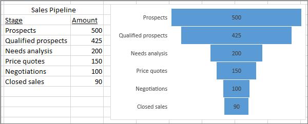
Funnel charts show values across multiple stages in a process. For example, you could use a funnel chart to show the number of sales prospects at each stage in a sales pipeline. Typically, the values decrease gradually, allowing the bars to resemble a funnel.
Enhanced Visuals
You can now insert what are known as Scalable Vector Graphics (SVG) files into not just Excel but any of your Microsoft Office documents, workbooks, emails and presentations. Once they're in place, they are easy to rotate, colour, filter and resize with no loss of image quality. To insert:
- Insert an SVG file in Office for Windows: simply drag and drop the file from Windows File Explorer into your document
- Insert an SVG file in Office for Mac: Go to Insert > Pictures > Picture from file to insert your SVG images.
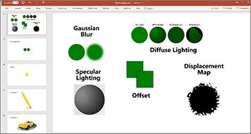
Further, you may transform all SVG pictures and icons into Office shapes so you can change their colour, size or texture:

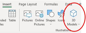
You can insert 3D models into your Excel files much the same way as other images. On the ‘Insert’ tab of the Ribbon, select 3D ‘Models’ and then ‘From a File’:
You can use 3D to increase the visual and creative impact of your, so that images may be rotated through 360 degrees.

Ink Improvements
We can’t say we use these features much in financial modelling, but some of you out there may. Inking features were initially introduced in Office 2016, but there have been improvements made in the 2019 counterpart:
- New ink effects: you can now express your ideas using metallic pens and ink effects like rainbow, galaxy, lava, ocean, gold, silver and more

- Digital Pencil: you may write or sketch out ideas with the new pencil texture
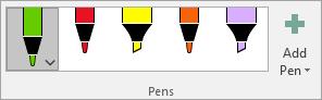
- Customisable, portable pen set: It’s now possible to create a personal set of pens to suit your needs. Office remembers your pen set in Word, Excel and PowerPoint across all of your Windows devices
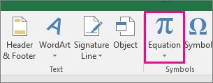
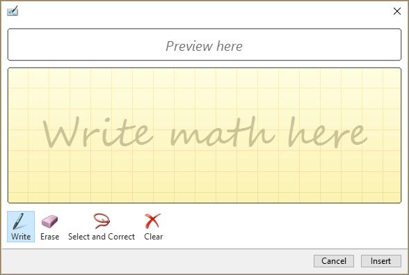
- Ink equations: including mathematical equations is now easier – simply go to Insert > Equation > Ink Equation, any time you want to include a complex maths equation in your workbook. If you have a touch device, you can use your finger or a touch stylus to write math equations by hand and Excel will convert it to text. (If you don't have a touch device, you can use a mouse to write, too.) You may also erase, select and correct what you've written as you go
Note to Microsoft: it’s “Maths”…
- New Ink Replay button: if you are using ink in your spreadsheets, you can now replay or rewind your ink to better understand the flow of it. This offers an alternative to GIF images to provide get step-by-step instructions. You'll find ‘Ink Replay’ on the ‘Draw’ tab
- Lasso Select at your fingertips: Excel now has Lasso Select
- a free-form tool for selecting ink. Drag with the tool to select a particular area of an ink drawing, and then you can manipulate that object as you wish
- Convert ink drawing to shapes: the ‘Draw’ tab lets you select inking styles and start making ink annotations on your touch-enabled device. You may also convert those ink annotations to shapes. Just select them and then select ‘Convert to Shapes’. That way, you get the freedom of freeform drawing with the uniformity and standardisation of Office graphic shapes
- Use your Surface pen to select and change objects: Well that assumes you have a Surface! In Excel, with a Surface pen, you can select an area without even tapping the selection tool on the Ribbon. Just press the barrel button on the pen and draw with the pen to make a selection. Then you can use the pen to move, resize or rotate the ink object.
Better Accessibility Features
Before sharing your spreadsheet, in Excel 2019 you can run the ‘Accessibility Checker’ to ensure your content is easy for people of all abilities to read and edit. On the Ribbon, click the ‘Review’ tab and then click ‘Check Accessibility’:
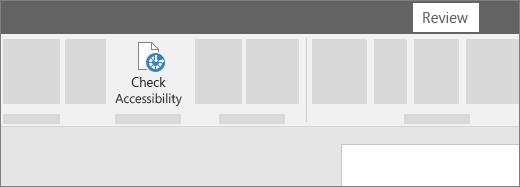
This will provide review results. You may see a list of errors, warning, and tips with how-to-fix recommendations for each. Excel 2019 now offers one-click fixes and is better than ever with updated support for international standards and handy recommendations to make your documents more accessible for all users.

Helpful sounds improve accessibility, but be careful: when you make changes to settings, the option affects all Microsoft Office programs that support this. Having said that, you can turn on audio cues to guide you as you work.
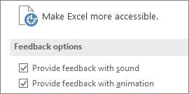
In the ‘File’ menu, select ‘Options’ (ALT + T + O). On the ‘Ease of Access’ tab, under ‘Feedback Options’, select or clear the ‘Provide feedback with sound checkbox’. If you wish, you can use the original Office sound effects by selecting the ‘Classic theme’ from the ‘Sound Theme’ drop-down.
Sharing and Saving
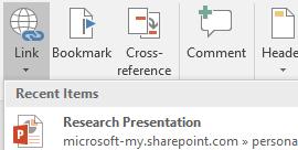
You can now attach hyperlinks to recent cloud-based files or websites and create meaningful display names for people using screen readers. To add a link to a recently used file, on the ‘Insert’ tab, choose ‘Link’ and select any file from the displayed list.
That’s not all. You may also view and restore changes in workbooks that are shared. You can now quickly view who has made changes in workbooks that are shared, and easily restore earlier versions.
Microsoft Office automatically saves versions of your SharePoint, OneDrive and OneDrive for Business files while you’re working on them (we have covered this before and not necessarily favourably!). These versions allow you to look back and understand how your files evolved over time and allow you to restore older versions in case you have made a mistake.
Version history in Office only works for files stored in OneDrive or SharePoint Online. If you don't see this option it's possible your file is stored in a different service or on a local device. To view historical versions:
- Open the file you were working on
- Click the File > Info and select ‘View and restore previous versions’
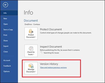
- The ‘Version history’ tab will open. Click a version to open and view it in a separate window.
With the version you want to restore open in your application, click ‘Restore’ in the message bar at the top of the opened version. Restore will save your current file as a new version and then replace your current file with the contents of the version you chose to restore.
You can quickly save to recent folders too. Go to File > Save As > Recent, and you’ll see a list of recently accessed folders that you can save to.
Selecting Only What You Want
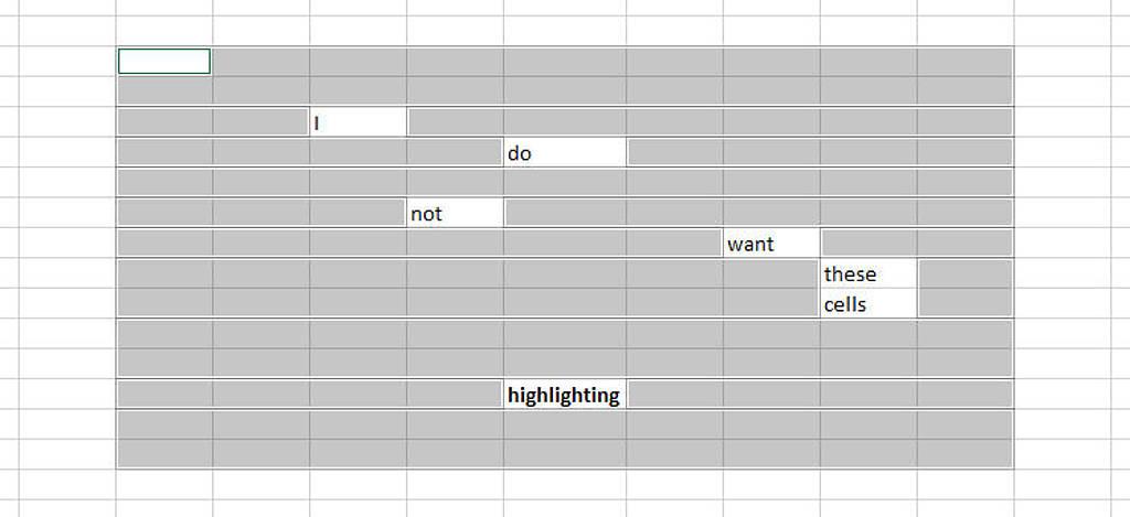
Excel will now let you deselect cells or a range of cells from your current selection. Microsoft has just rolled this out for PC and Mac subscription users of Office 365.
To "unselect" (it's a new word, look it up!) a selected cell, hold down the CTRL button (or Command on a Mac) key and click on the cells you want to deselect. To unselect a range of selected cells, hold down the CTRL (or again, the Command for Mac) key and drag the range you want to deselect, starting from within the selected range.
Don’t get confused with the cell in the top left-hand corner of the range selected remaining white! You can have fun experimenting what that looks like when it is de-selected...
Quick Access to Superscript and Subscript
Now this one made me laugh. This is apparently a new feature, but we swear you have been able to do this since the Quick Access Toolbar came out! You can now add these features to the Quick Access Toolbar. Wow.
There you go. If ever there was a business case to go out and buy Excel 2019, that certainly wasn’t it…
Improved AutoComplete
Microsoft has improved the AutoComplete functionality in that you no longer need to be so precise to find what you are looking for, e.g.
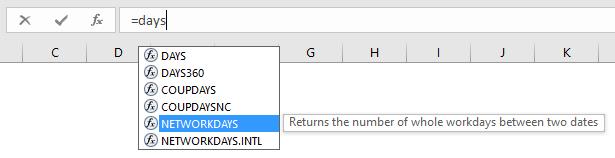
Excel will now look for functions or range names that contain the phrase sought. This will help immensely when you cannot quite remember what it was you are looking for. This one is cool.
New Themes
There are now three Office Themes that you can apply: Colorful (sic), Dark Gray and White. To access these themes, go to File >Options > General, and then click the drop-down menu next to ‘Office Theme’.
Black Theme
The highest-contrast Office theme yet has arrived. To change your Office theme, go to File > Account, and then click the drop-down menu next to Office Theme. The theme you choose will be applied across all your Office apps.
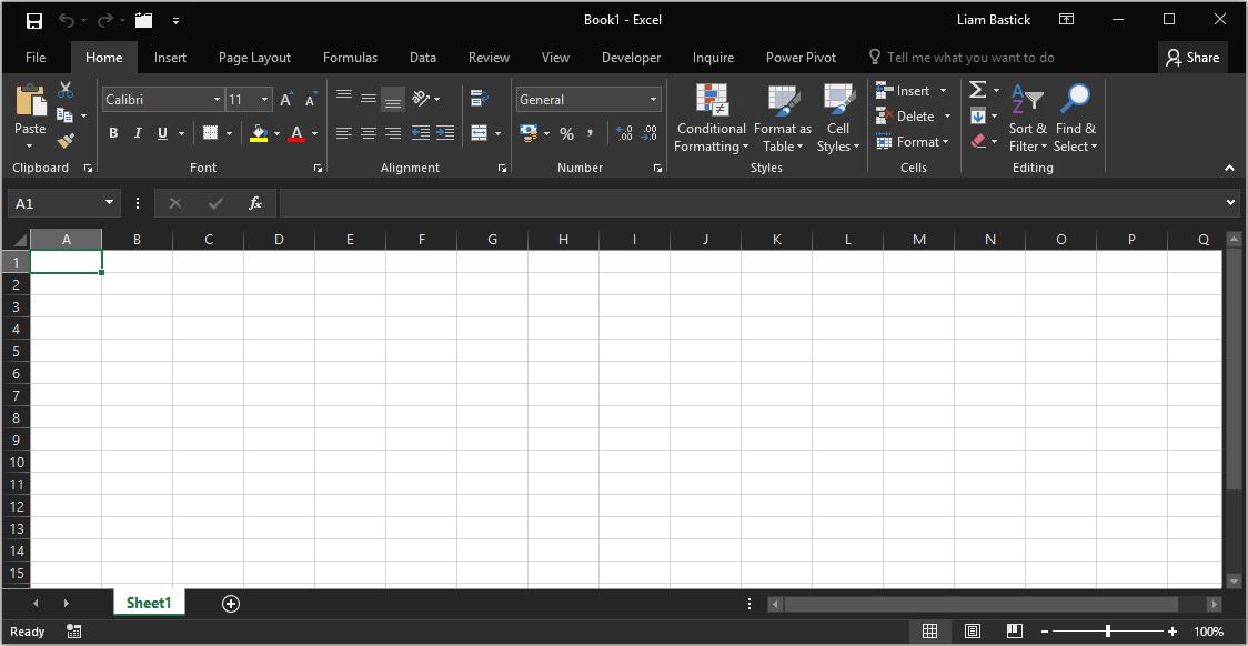
Perfect for hangovers and for reflecting your mood when you have to work late, we originally claimed we weren’t quite sure this was going to catch on, but we have seen many clients adopt this. I suppose once you go black you never go back…
Translator
Translate words, phrase, or sentences to another language with Microsoft Translator. You can do this from the ‘Review’ tab in the Ribbon:

CSV Improvements
Remember this warning: "This file may contain features that are not compatible with CSV..."? Well, apparently no one wanted it. So Microsoft has got rid of it when you save a CSV file.
Furthermore, you can now open and save CSV files that use UTF-8 character encoding. Go to File > Save As > Browse. Then click the ‘Save as type’ menu, and you'll find the new option for ‘CSV UTF-8 (Comma delimited)’. CSV UTF-8 is a commonly used file format that supports more characters than Excel’s existing CSV option (ANSI). What does this mean in English? Better support for working with non-English data, and ease of moving data to other applications.
Data Loss Protection (DLP) in Excel
Data Loss Protection (DLP) is a high-value enterprise feature that is well loved in Outlook. Now it is being introduced into Excel to enable real time scan of content based on a set of predefined policies for the most common sensitive data types (e.g. credit card numbers, social security numbers and [US] bank account numbers).
This capability will also enable the synchronisation of DLP policies from Office 365 in Excel, Word and PowerPoint, and provide organisations with unified policies across content stored in Exchange, SharePoint and OneDrive for Business.
PivotTable Enhancements
PivotTables were enhanced beyond recognition with the advent of Excel 2010 and Excel 2013, and the introduction of Power Pivot and the Data Model, bringing the ability to easily build sophisticated models across your data, augment them with measures and KPIs and then calculate over millions of rows with high speed. But it’s not stopped there:
- Personalise the default PivotTable layout: you may now set up a PivotTable the way you like. You can choose how you want to display subtotals, grand totals and the report layout, then save it as your default. This means that the next time you create a PivotTable, you will start with that layout
- Automatic relationship detection: this feature discovers and creates relationships among the tables used for your workbook’s data model, so you don’t have to. Excel knows when your analysis requires two or more tables to be linked together and notifies you. With one click, it does the work to build the relationships, so you can take advantage of them immediately
- Creating, editing, and deleting custom measures: this may now be done directly from the PivotTable fields list, saving you a lot of time when you need to add additional calculations for your analysis
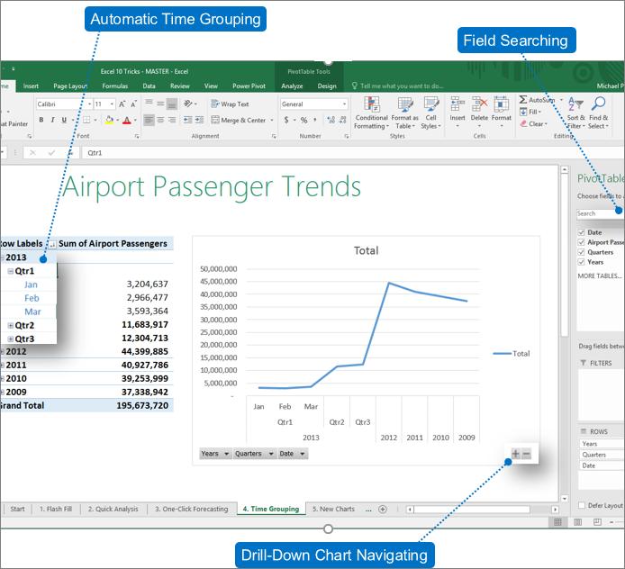
- Automatic time grouping: this helps you to use time-related fields (year, quarter, month) in your PivotTable more powerfully, by auto-detecting and grouping them on your behalf. Once grouped together, simply drag the group to your PivotTable in one action and immediately begin your analysis across the different levels of time with drill-down capabilities
- PivotChart drill-down buttons: this allows you to zoom in and out across groupings of time, and other hierarchical structures within your data
- Search in the PivotTable: the ‘Field list’ helps you get to the fields that are important to you across your entire data set
- Smart renaming: this gives you the ability to rename tables and columns in your workbook’s data model. With each change, Excel automatically updates any related tables, and calculations across your workbook, including all worksheets and DAX formulae. This is quite a welcome improvement as this caused many problems in previous versions of Excel
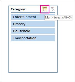
- Multi-select Slicer: you may now select multiple items in an Excel Slicer on a touch device. This is a change from prior versions of Excel, where only one item in a Slicer could be selected at a time using touch input. You can enter Slicer multi-select mode by using the new button located in the Slicer’s label
- Faster OLAP PivotTables: if you work with connections to online analytical processing (OLAP) servers, your PivotTables are now faster. Excel 2019 contains query and cache improvements in this powerful feature’s performance. You could benefit from this work, whether you use PivotTables to answer one-off questions, or build complicated workbooks with dozens of PivotTables. It doesn’t matter if your PivotTables are connected to a tabular or multi-dimensional model. Any PivotTable connected to Microsoft SQL Server Analysis Services, third party OLAP providers or the Power Pivot Data Model will likely give you fresh data, faster. Additionally, now if you disable Subtotals and Grand Totals, PivotTables can be much faster when refreshing, expanding, collapsing, and drilling into your data. The bigger the PivotTable, the bigger the potential improvement. Specifically, Excel 2019 offers improvements in three major areas while querying OLAP servers:
- Improved query efficiency: Excel will now query for Subtotals and Grand Totals only if they’re required to render the PivotTable results. This means you wait less for the OLAP server to finish processing the query and you wait less while waiting for the results to transfer over your network connection. You simply ‘disable Subtotals and Grand Totals’ from the ‘PivotTable Design’ tab just like you would normally
- Reduced the number of queries: Excel is smarter when refreshing your data. Queries will now only refresh when they’ve actually changed and need to be refreshed
- Smarter caches: when the PivotTable schema is retrieved, it is now shared across all of the PivotTables on that connection, further reducing the number of queries.
Power Pivot Updates
Power Pivot gets a dusting down in Excel 2019 too:
- Save relationship diagram view as picture: you may now save the data model diagram view as a high resolution image file that can then be used for sharing, printing or analysing the data model. To create the image file, in the ‘Power Pivot’ pane, click File > Save View as Picture
- Multiple usability improvements: these have also been made. For example, delayed updating allows you to perform multiple changes in Power Pivot without the need to wait until each is propagated across the workbook. The changes will be propagated at one time, once the Power Pivot window is closed.
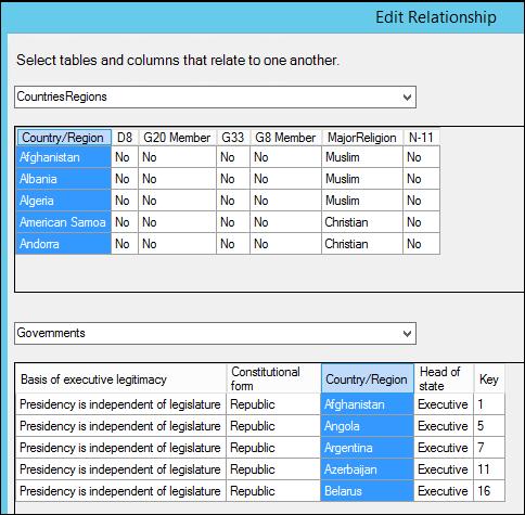
- Enhanced ‘Edit Relationship’ dialog creates faster and more accurate data relationships: Power Pivot users can manually add or edit a table relationship while exploring a sample of the data—up to five rows of data in a selected table. This helps create faster and more accurate relationships, without the need to go back and forth to the data view every time you wish to create or edit a table relationship
- Table selection using keyboard navigation: in the ‘Edit Relationship’ dialog, type the first letter of a table name to move the first column name starting with the selected letter
- Column selection using column navigation: in the ‘Edit Relationship’ dialog, type the first letter of a column name to move the first column starting with the selected letter. Retype the same letter moves to the next column starting with the selected letter
- Auto column suggestion for same column name in both tables: after selecting the first table and column, on the selection of the second table, if a column with the same name exists, it is auto-selected (works both ways)
- Fixes that improve your overall modelling user experience:
- The Power Pivot data model is no longer lost when working with hidden workbooks
- You can now upgrade an earlier workbook with a data model to Excel 2016 and later
- You can add a calculated column in Power Pivot, unless it contains a formula.
Get & Transform (Power Query)
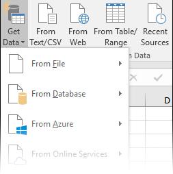
Improvements have also been made to Get & Transform (also known as Power Query):
- New and improved connectors: there are now new connectors in Excel 2019. For example, there's the new SAP HANA connector. Excel 2019 has also improved many of the existing connectors so that you can import data from a variety of sources with efficiency and ease
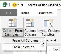
- Improved transformations: in Excel 2019, Microsoft has significantly improved many of the data transformation features in the Power Query Editor. For example, splitting columns, inserting custom columns, adding columns from an example, merge and append operations, and filtering transforms have been improved / enhanced
- General improvements: Excel 2019 also has some general improvements across the Get & Transform area in Excel 2019. One notable improvement is the new ‘Queries & Connections’ side pane, which lets you manage queries and connections easily. There are also many improvements to the Power Query Editor as well, including “select-as-you-type” drop-down menus, date picker support for date filters and conditional columns, the ability to reorder query steps via drag-and-drop and the ability to keep the layout in Excel when refreshing.
Publish to Power BI
If you have a Power BI subscription, you can now publish files that are stored locally to Power BI. To get started, first save your file to your computer. Then click File > Publish > Publish to Power BI. After you upload, you can click the ‘Go To Power BI button’ to see the file in your web browser.
Finally, one thing to stress. Excel 2019 is what is known as a “perpetual licence”. Microsoft will update for security features and so forth but new features – described here in past newsletters – such as Dynamic Array functions will not be included down the road. It’s likely you will have to wait until Office 2022 (assuming such a thing will exist) as Microsoft tries to convert everyone to the annual subscription model.