New Improved RANDARRAY Function Coming Soon to Office 365 Excel

OK, so this is still in what Microsoft refers to as “Preview” mode, i.e. it’s not yet “Generally Available” but it is on the outskirts of civilisation. RANDARRAY is still a relatively new function found in some editions of the “Office Insider” programme which is an Office 365 fast track. You can register in File -> Account -> Office Insider in Excel’s backstage area.

Even then, you’re not guaranteed a ticket to the ball as only some will receive the new features as Microsoft slowly roll out these features and functions.  Please don’t let that put you off.  These features will be with all Office 365 subscribers soon.

We first mentioned RANDARRAY back in September.  Even though it’s not yet Generally Available, it’s already had a facelift.  Oh yes – Microsoft is invested in these functions!

Originally, the RANDARRAY function returned an array of random numbers between 0 and 1.  It’s not clear from Microsoft, analogous to the pre-existing RAND function, which generates a number greater than or equal to zero and strictly less than one.  However, there was a general sense of underwhelm with this function and the new and improved version has just been released.  It now allows you to set you own maximum and minimum and decide whether you want the values returned to be decimals (e.g. 17.4381672…) or integers (whole numbers).

The new syntax for the function is now as follows:

The function has five arguments, all supposedly optional (but upon testing, we weren’t quite as convinced):

• rows: this specifies how many rows the results should spill over.  If omitted, the default value is 1
• columns: this specifies how many columns the results should spill over.  If omitted, the default value is also 1
• min: this is the minimum value that may be selected randomly.  If this is not specified, it is assumed to be zero (0)
• max: this is the maximum value that may be selected randomly.  If this is not specified, it is assumed to be 1
• integer: if this is set to TRUE, only integer outputs are allowed; the default value (FALSE) provides non-integer (decimal) results.

Other points to note:

• if rows or columns refers to a blank cell reference, this will generate the new #CALC! error
• if rows or columns are entered as decimals, the values used will be truncated to the number before the decimal point (e.g. 3.999 will be treated as 3 digits)
• if rows or columns is a value less than 1, #CALC! will be returned
• if integer is set to TRUE and either min or max is not an integer, this will generate an #VALUE! error
• max must be greater than or equal to min, else the error #VALUE! is returned.

When we originally discussed the RANDARRAY function, we used this rather comprehensive example to create a list of random integers between two values:

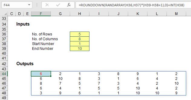
Originally, the formula in cell F44 was

and the article explained how this worked.  However, it’s much easier now:

The “new improved” formula in cell F45 (it’s moved down a row due to the additional argument required in cell H40) is simply

Cool, eh?