VBA Blogs: Charts and Macros 4

Welcome back to this week’s VBA blog!  This month, we have been looking at the interaction between charts and macros.

As we mentioned previously, this month we’re going to look at the thought process around creating a macro that would help us to identify a chart’s details and present the results to a user.  We effectively need to go through the following steps:

• Define the target / output file, save target details
• Determine the series details and loop through to extract them
• Extract out the relevant name / y-axis / x-axis / bubble size from the formula and clean up

This week, we’re covering the final step in that list.

So far, we’ve extracted out details from the charts in a workbook and dropped them into a new workbook that looks something like this:

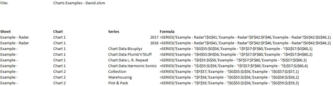
From here, we need to disentangle the formula to work out what the component parts of the data series are.  Luckily, there are a few basic rules:

• The formula always starts off with “=SERIES(“
• The name of the data series will the first parameter (i.e. before the first comma)
• It’s always followed by the Y-axis, the X-axis, any bubble size or Z-axis (where relevant)
• It finishes off with a number indicating where in the list of series items it is.

As a result, we can use formulae to work out what each component is.  So under the Name column, we can use the following formula to extract the name:

We can then repeat the steps for the axis items as well:

All of these formulae basically look up the location of the relevant commas and brackets in order to find the start and end points of each of the chart series details.  In order to build them into the code, we need something like this:

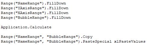
Once the formulae are in place, we can copy these down, then copy and paste-special as values, so that we don’t have the formulae there the whole time – it’s much easier to follow if it’s hard-coded.

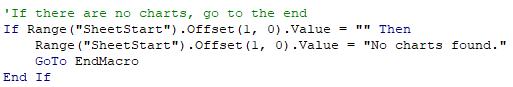
There’s another thing too – if there are no charts in the workbook, the formulae will simply break.  In that instance, we might just want a simple message that lets the user know that there are no charts.

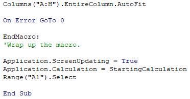
Then, all that is left is a bit of macro clean-up to tidy things up and reset screen updating and calculation statuses.

And that’s it – that’s our full macro! You can find a sample of the whole thing here - have a play around and let us know what you think. Next week is the Final Friday Fix, so we’ll be back next month with more VBA tricks. See you then!