
Power Query: Split Folder Part 7
14 May 2025
Welcome to our Power Query blog. This week, I extract the parameters from the Excel workbook.
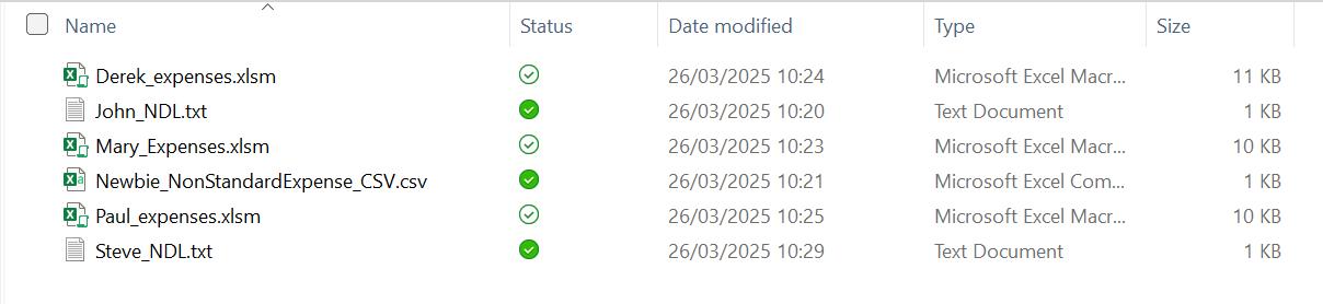
I have covered the topic of getting files from a folder in several blogs; the latest series was Excel Files from a Folder Fiddle. In this series, I will look at how I may extract files from a folder, where some of the files require different transformations to others. The folder shown below contains expense data for May 2024, but not all formats are the same:
My task is to transform all the data and append into a single output Table.
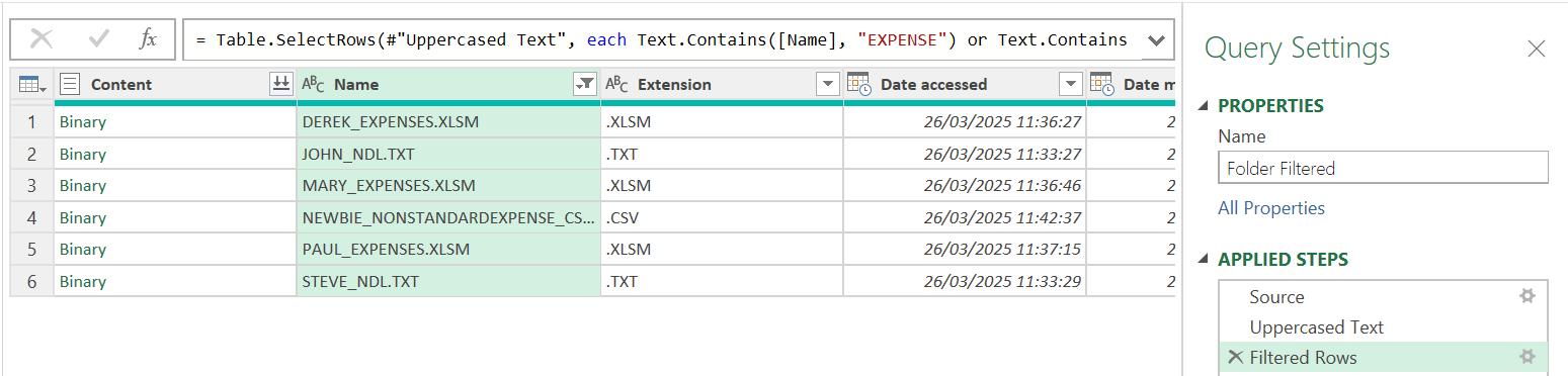
In Part 1, I used the ‘From Folder’ connector to extract data from the folder and transformed / filtered the data to ensure I only had the expense data.
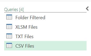
I took three [3] reference copies of Folder Filtered, one for each file type:
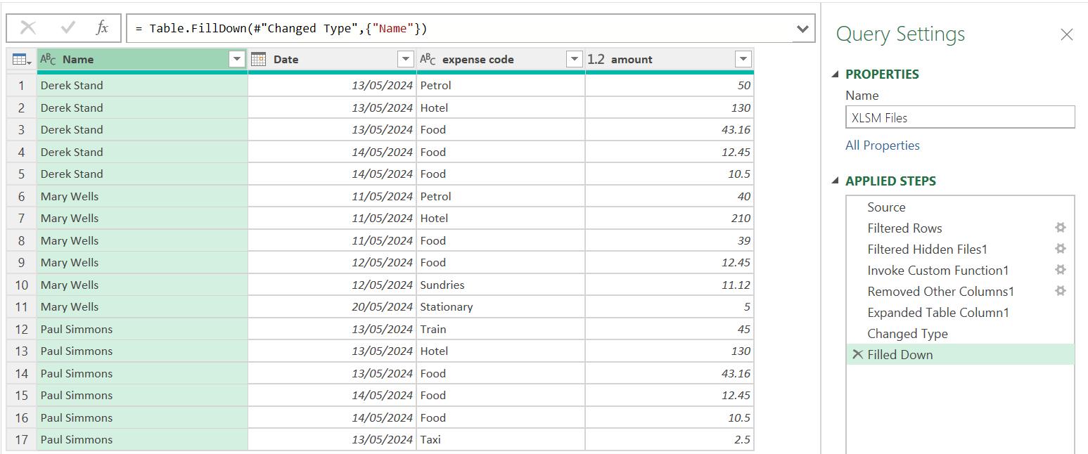
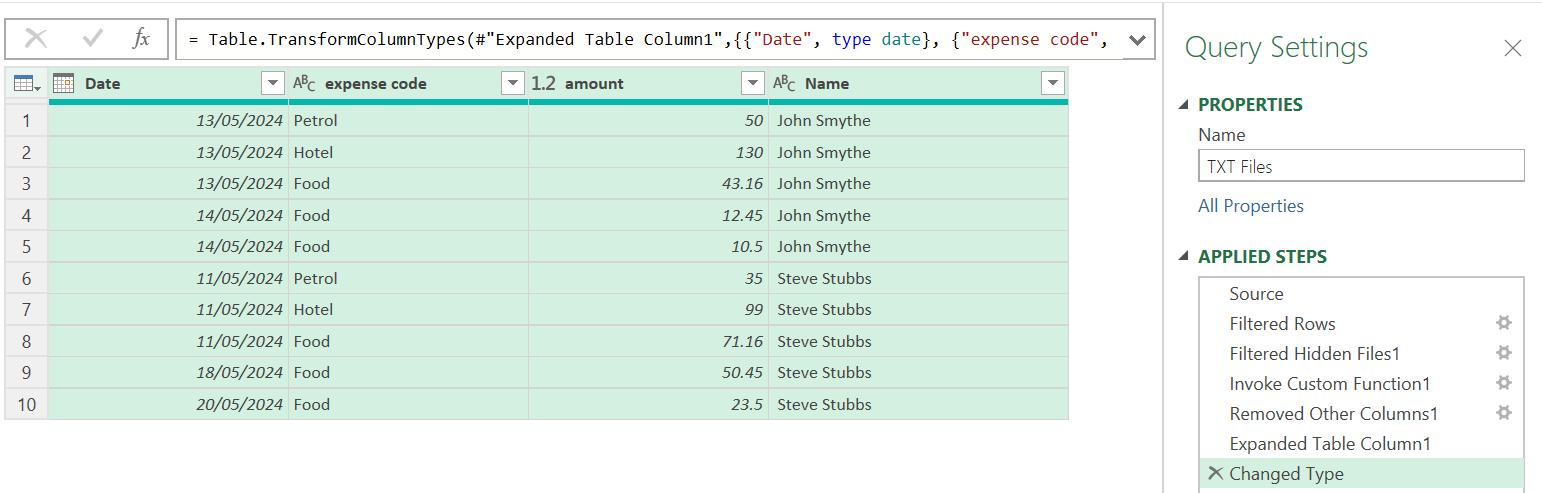
In Part 2, I transformed the data in XLSM Files and TXT Files.
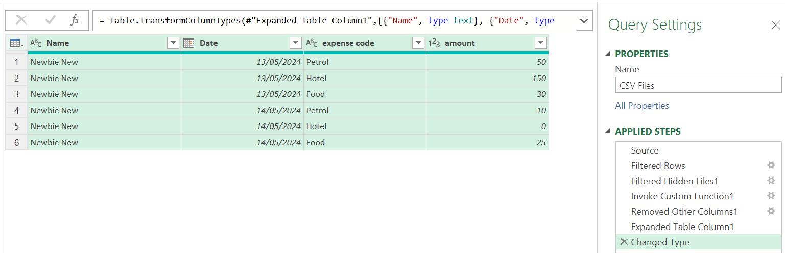
In Part 3, I transformed the CSV Files. Currently, there is only one CSV file, but I assume that there could be more when I refresh the data, so I used the ‘Combine Files’ approach.
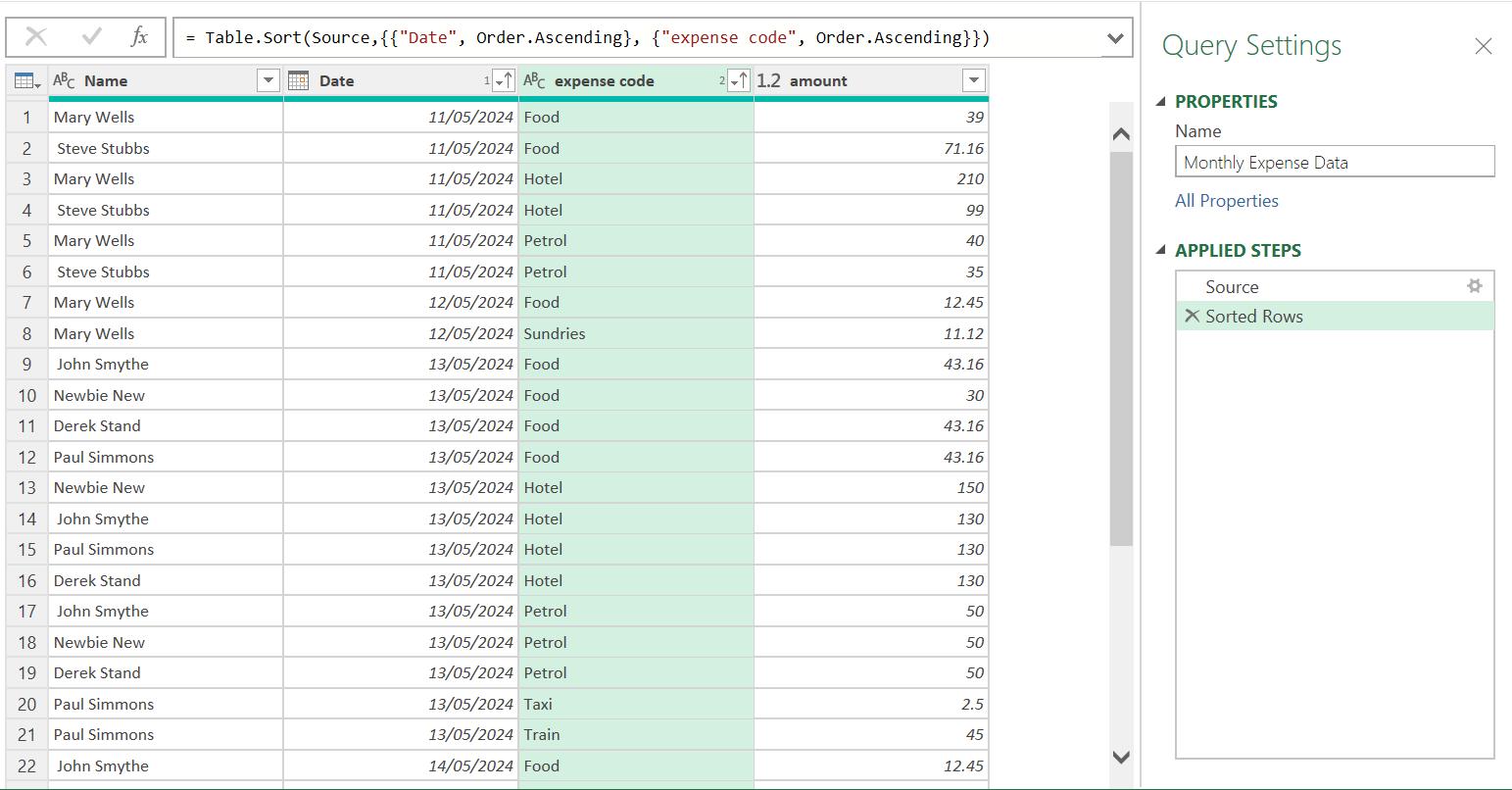
I appended my data to create a new query Monthly Expense Data, and sorted the data in ascending Date order:
In Part 4, I tested the process by changing and adding data.
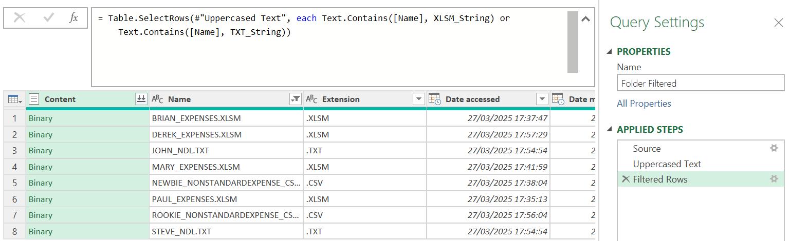
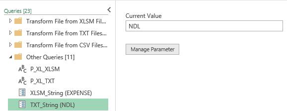
In Part 5, I refined the process by using internal Power Query parameters in the Folder Filtered query.
The values of the parameters were "EXPENSE" and "NDL".
When I clicked OK, the query looked the same, but I was using parameters for the 'Filtered Rows' step:
Last time, I investigated what happened if there wasn't a file selected of each type and I changed the queries XLSM Files, TXT Files and CSV Files to always have at least one row and changed Monthly Expense Data, so that it would ignore the extra column and null row that the solution could produce.
Whilst having internal Power Query parameters is better than hard coding, this is only suitable for users who are comfortable using Power Query. This time, I'll look at getting the data from the Excel worksheet instead.
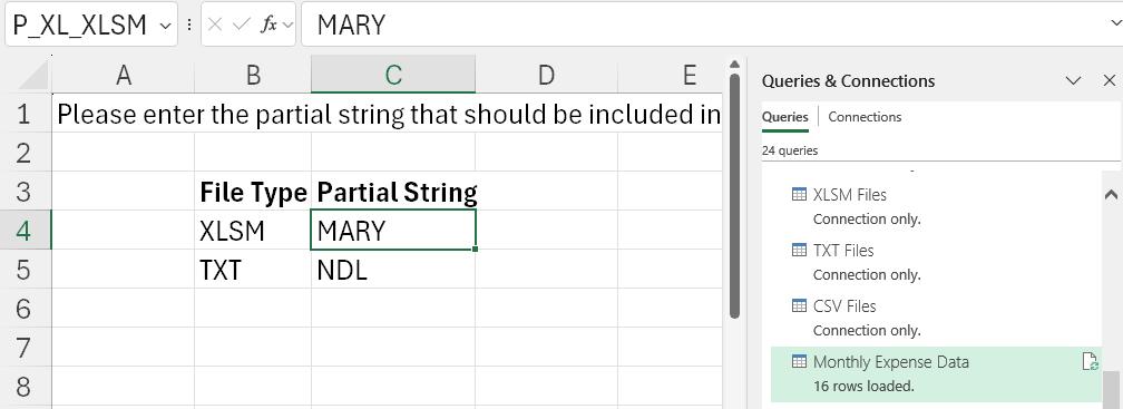
On a new worksheet, which I call 'Inputs', I create two labels and two named ranges.
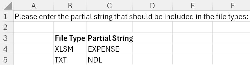
The named ranges are P_XL_XLSM and P_XL_TXT. I right-click on cell C4, and choose to 'Get Data from Table/Range':
This gives me a new query P_XL_XLSM:
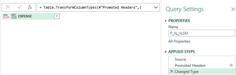
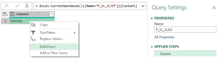
I don't want the default steps, so I delete 'Changed Type' and 'Promoted Headers'. I right-click on the cell and choose to 'Drill Down':
This gives me a single value for P_XL_XLSM:
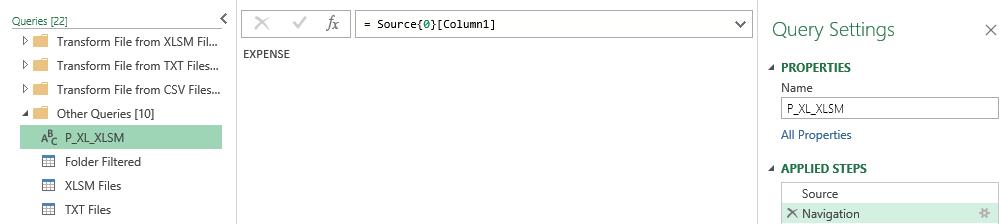
I repeat this process for P_XL_TXT:
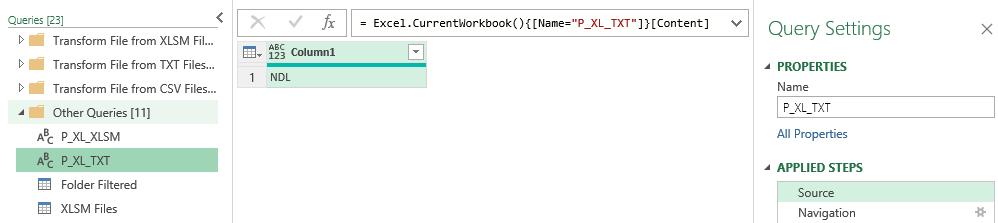
Since these queries each contain one data item, the icon is text. Note that they do not look like the parameters I created in Part 5.
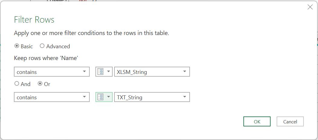
If I go back to the Folder Filtered query and use the cog next to the 'Filtered Rows' step, I am not able to select the parameters from the Excel worksheet:
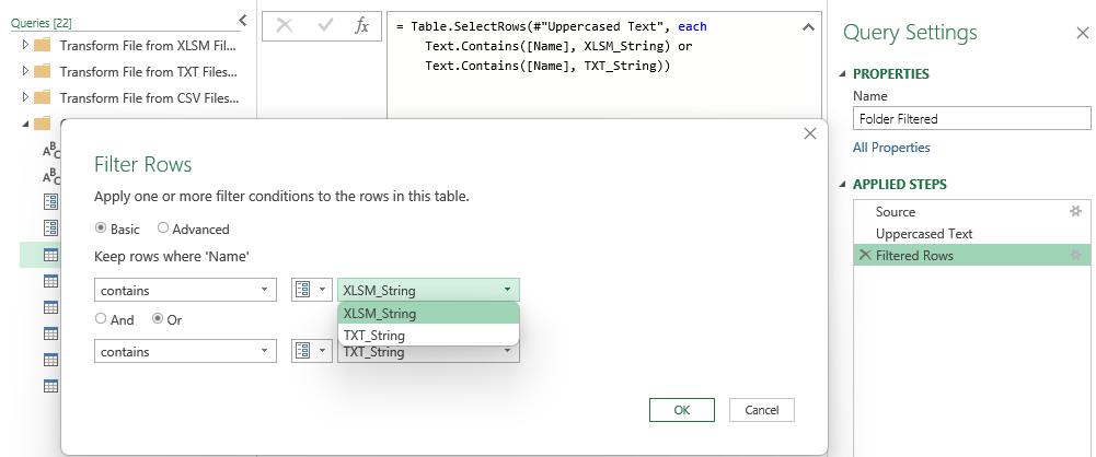
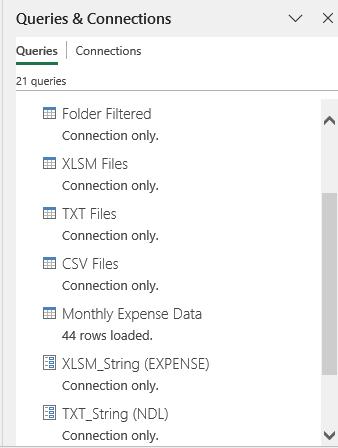
To use these filters, I must adjust the M code in the step instead. I change it from:
= Table.SelectRows(#"Uppercased Text", each Text.Contains([Name], XLSM_String) or Text.Contains([Name], TXT_String))
to
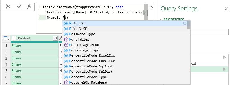
= Table.SelectRows(#"Uppercased Text", each Text.Contains([Name], P_XL_XLSM) or Text.Contains([Name], P_XL_TXT))
Note that the IntelliSense does recognise the new parameters:
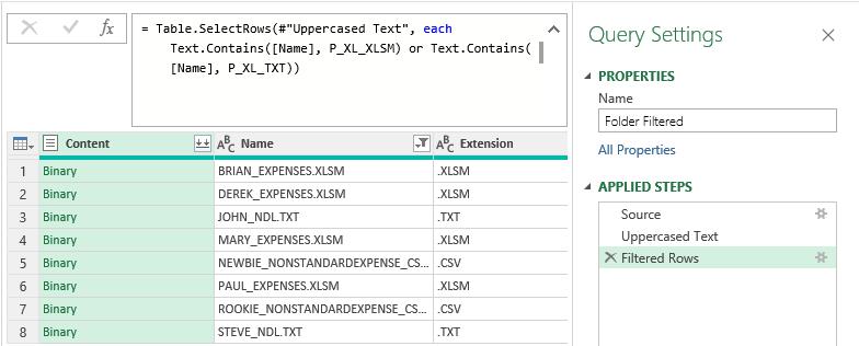
The output remains the same:
If the user changes one of the values in the 'Inputs' sheet, the filter changes when the query is refreshed:
This will make the process easier for the users to change, but it does leave the question: why can't I pick the parameters I have created in the 'Filtered Rows' step? Is there a way to make these parameters look like Power Query parameters so we can select them? Yes, there is, and I'll cover this next time.
Come back next time for more ways to use Power Query!