Power Query: Row Together Part 6

Welcome to our Power Query blog.  This week, I continue a new row challenge.

Over the last few weeks, I have been looking at how to solve tasks involving the manipulation of data to form new rows.  Last week, I began a slightly different version of the challenge.  The data I am  transforming is in an Excel Table SalesResults.

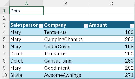
I have a list of amounts accrued by each Salesperson for our suppliers.  The task is to create a row for each Salesperson for each Company they have sold to detailing the total Amount, viz.

Last week, I extracted the data to a new query SalesResults:

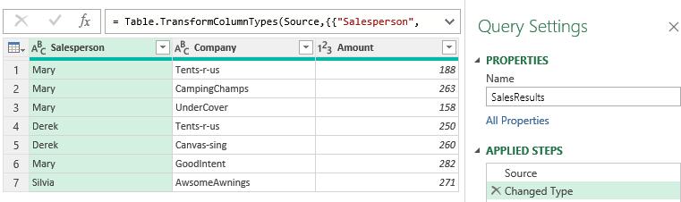
I sorted the data in ascending Salesperson order and created an index before grouping the data.

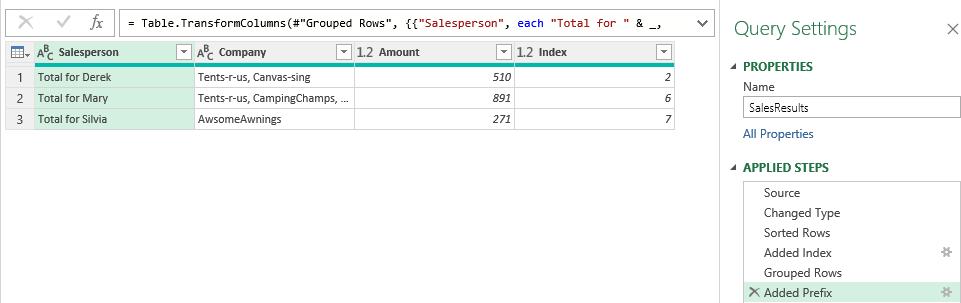
I amended the M code to aggregate the Company rows correctly and now I have the total rows:

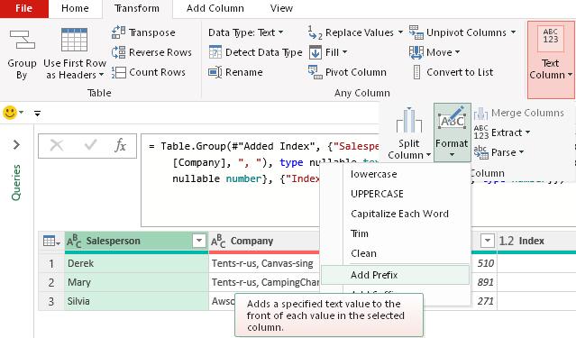
There are a few more changes I need to make to the total rows.  I need to format the Salesperson column to include the prefix "Total for ".  I can do this from the Transform tab.  In the 'Text Column' group there is a Format dropdown where I can 'Add Prefix':

Choosing this option opens the following dialog:

The data in Salesperson is now displayed correctly.

The next change I need to make is to the Index column.  Currently, it has the same value as the last row for each Salesperson.  I need to add a number to each value in Index so that it will appear in the correct position.  I can do this from the Transform tab.  In the 'Number Column' section, there is a Standard dropdown:

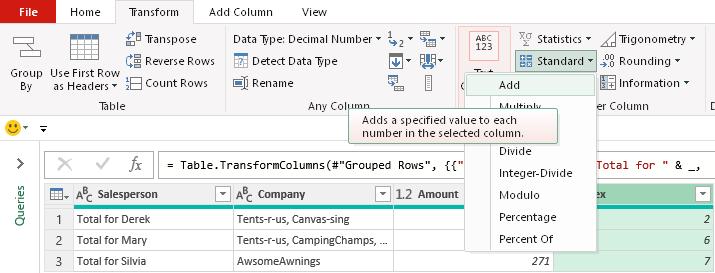
I can add a specified value to each number in the selected column.  When I choose this option, I access a dialog:

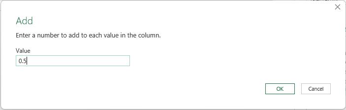
If I add one [1] to each Index, it would be part of the data group for the next Salesperson.  I need a value that is more than zero [0] but less than one.  I choose a half [0.5] and click OK.

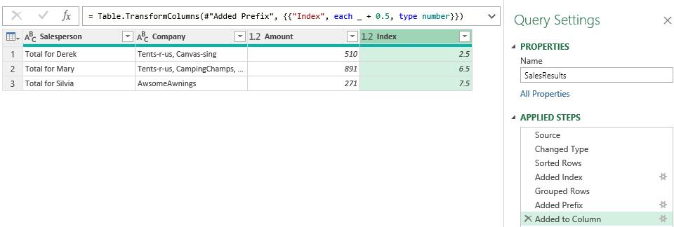
My data is ready for the next step, which is where I will continue next week.

Come back next time for more ways to use Power Query!