
Power Query: X Marks the Spot - Unleashed
16 May 2018
Welcome to our Power Query blog. This week, I look at a more comprehensive method to convert a check box into a name.
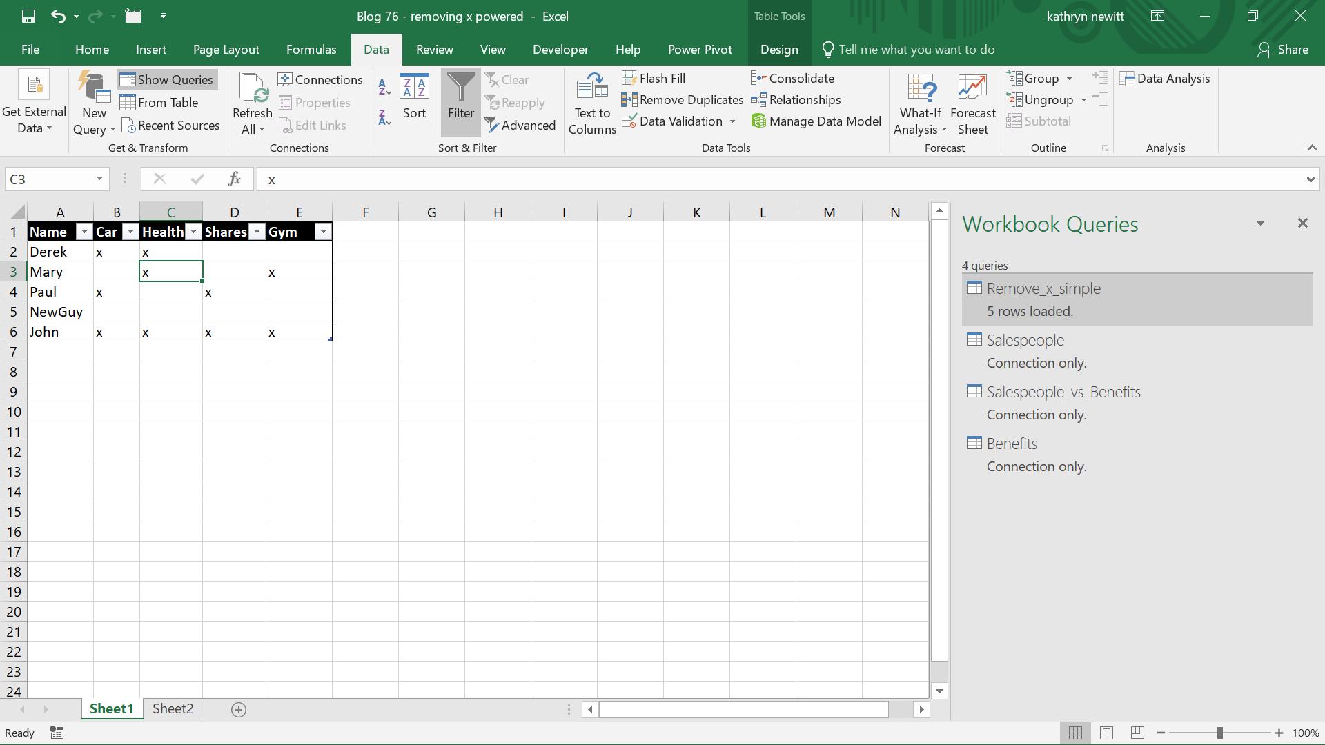
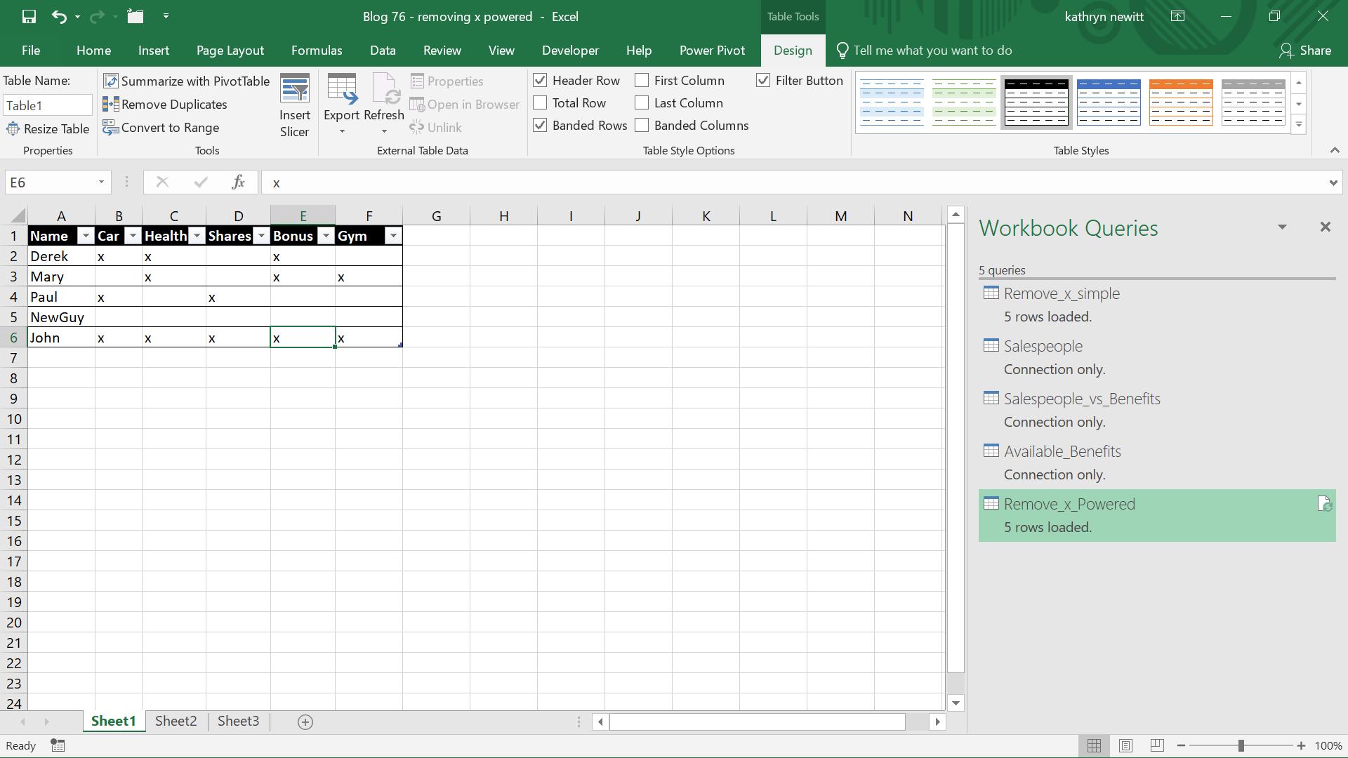
As for last week’s blog, my aim is to take the table below and transform it into a more useful layout.
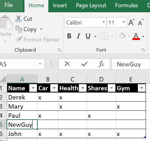
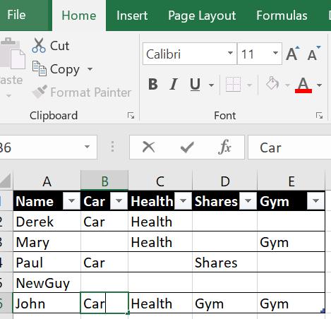
I am using the same simple table showing the usual imaginary salespeople and the benefits they may access. I have the same goal as last week; I want to end up with the layout below:
Last time, I looked at a way to achieve this on a small scale, by adding new columns. This time, I will look at a more complex version that will work for any number of columns.
In order to construct my table in the format that I require, I will first break it up into its constituent parts – Salesperson Name and Benefit types (i.e. a list of all the headings). I will also create a list of pairings between salespeople and benefits received. Finally, I can recreate my table, not forgetting that I also need to show which benefits are not received (this is particularly appropriate for poor ‘NewGuy’!).
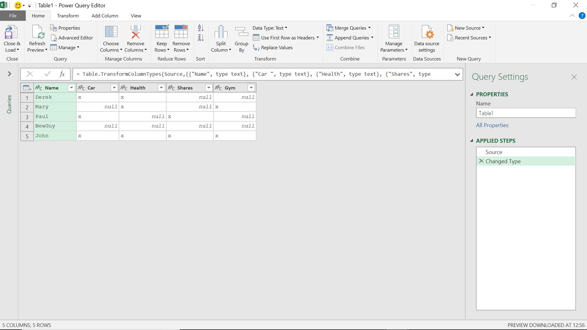
I create my query using ‘From Table’ on the ‘Get and Transform’ section of the ‘Data’ tab:
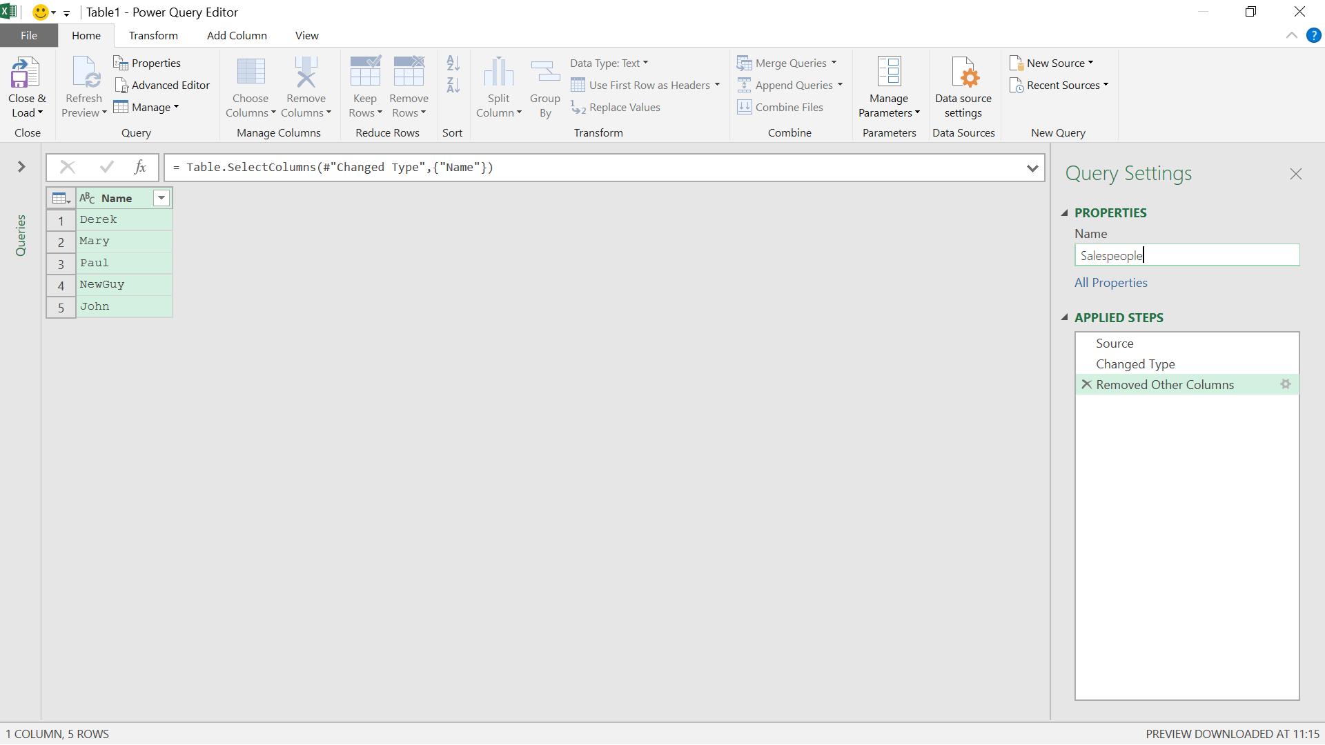
My first step is to obtain a list of salespeople, so I select the Name column and choose to ‘Remove other Columns’ from the ‘Remove Columns’ dropdown in the ‘Manage Columns’ section on the ‘Home’ tab. Note that in most cases, the functions used in this example are also available by right clicking on the appropriate column.

I have my first query, which I call ‘Salespeople’.
I save this query as ‘Connection Only’ as I will be using it to build my final query.
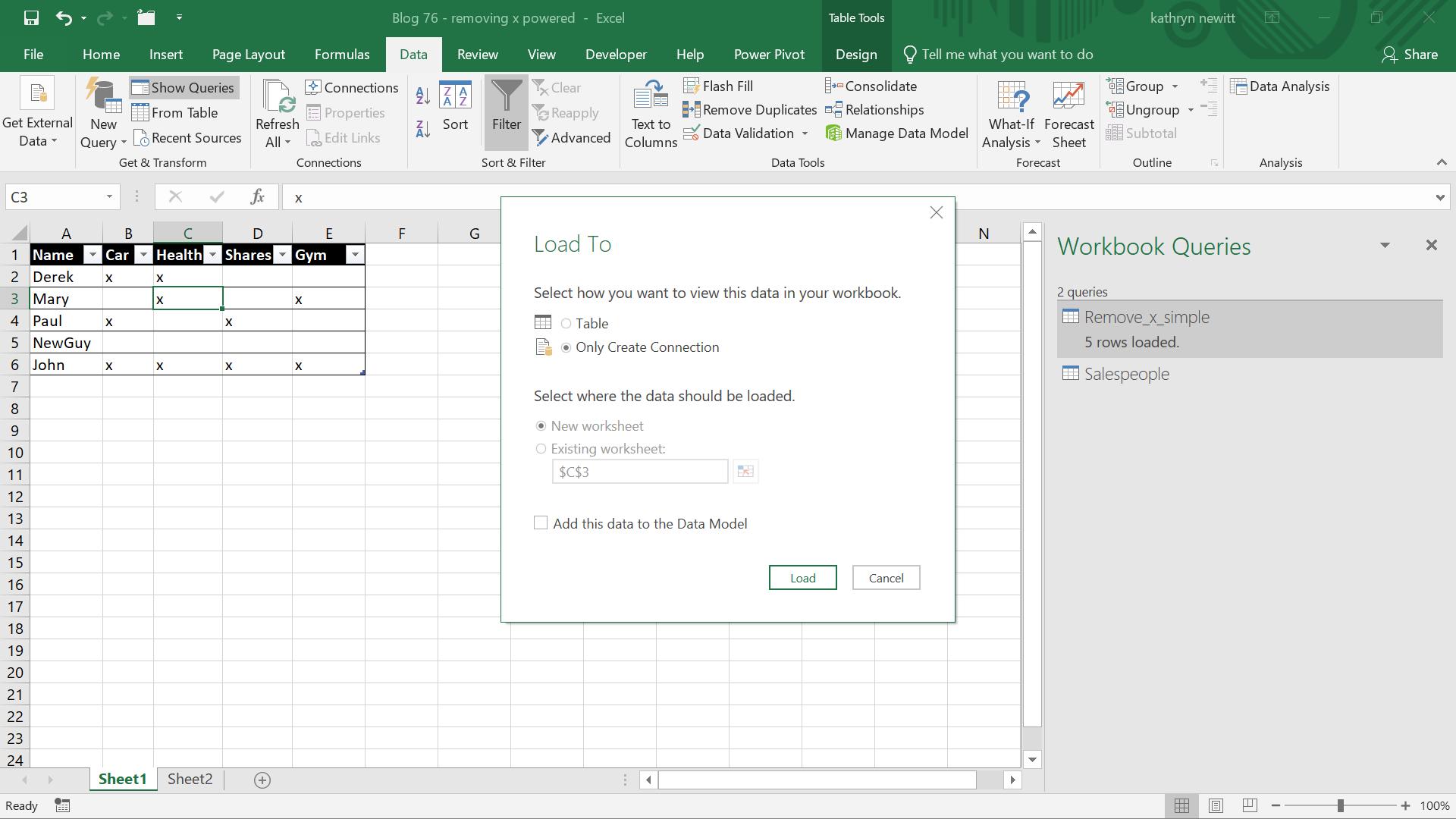
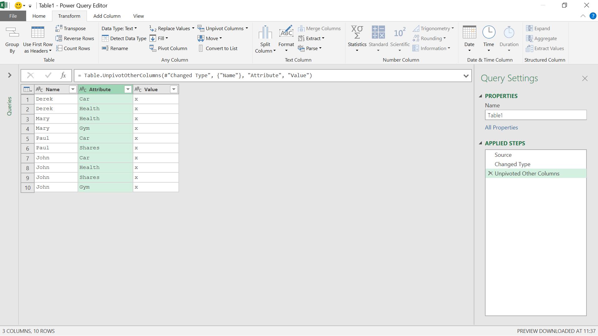
Now I need the next part of the data – a list of pairs to show each benefit a salesperson receives. I start my query in the same way as before from the table, but this time I need to unpivot my data. On the ‘Transform’ tab, having selected my Name column, I can choose to ‘Unpivot Other Columns’ from the ‘Unpivot Columns’ drop down in the ‘Any Column’ section.
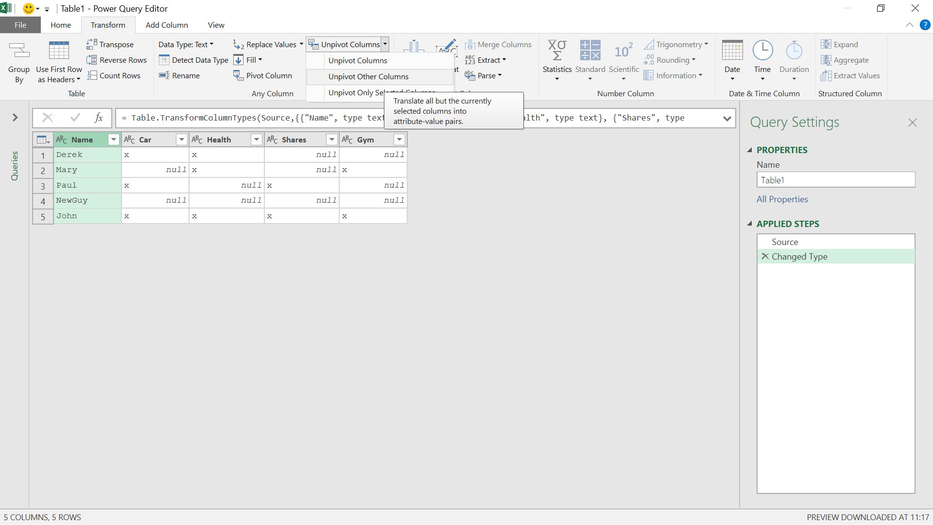
This gives me a list of salespeople and each benefit they receive. Note that ‘NewGuy’ is not shown because no values existed in the unpivoted columns for them. All the null cells, which had no ‘x’ in them, have been removed as part of the unpivoting process.
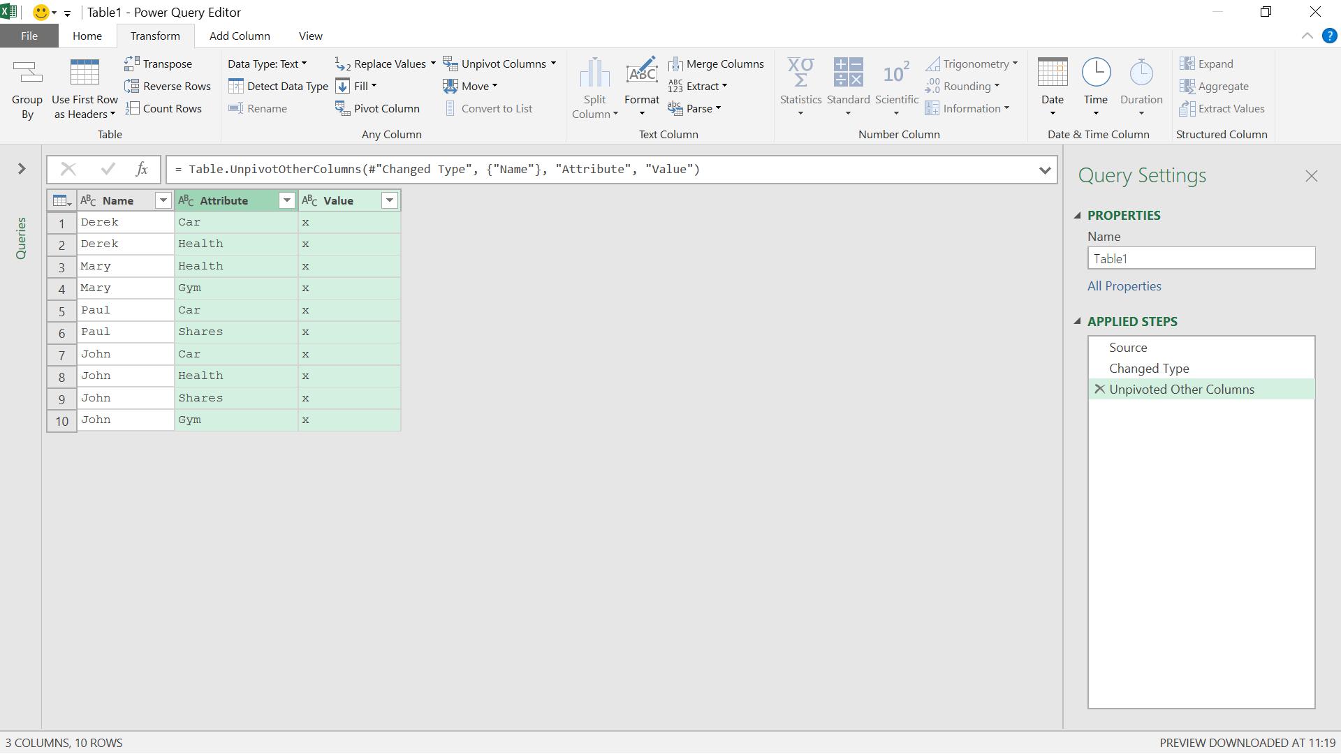
I can now delete the Value column and rename my query, which I also ‘Close & Load’ to ‘Connection Only’.
Thus, I have a list of salespeople and a list of benefits that each salesperson receives. I am now going to construct a list of the benefits that are available. I start again from my original table, and unpivot everything except the name again.
This time I am going to only keep the Attribute column, and ‘Remove Duplicates’ from ‘Remove Rows’ dropdown on the ‘Home Menu’, viz.
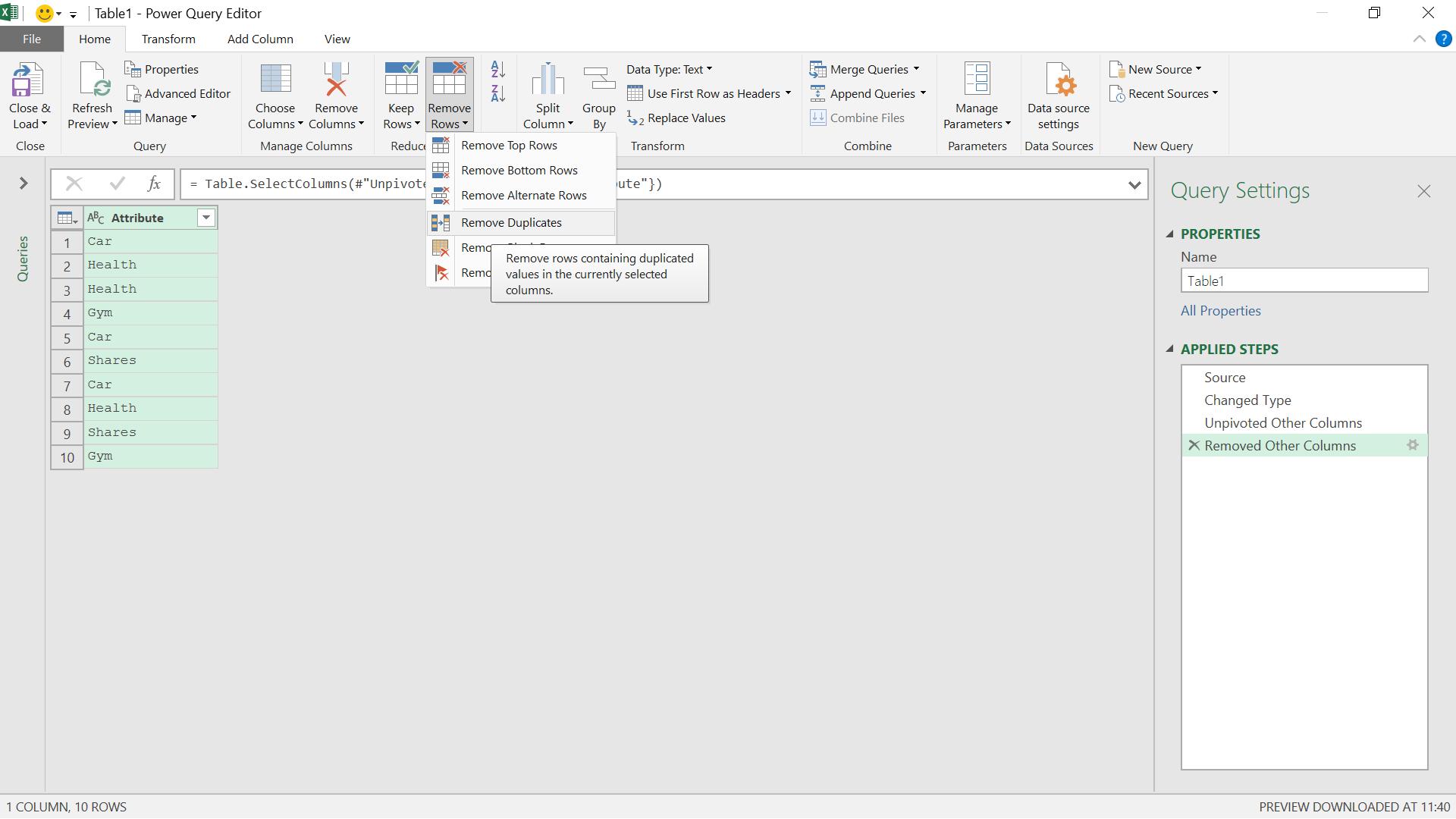
I now have a list of benefits, which I also save as ‘Connection Only’. I will call this query ‘Benefits’.
Now I have my building blocks, I can create my final query.
I start with my ‘Benefits’ query – I need to pull the salespeople back into this query, so I am going to add a custom column. The method I am using is a cross join, which I looked at in Power Query: Hot Cross Joins.
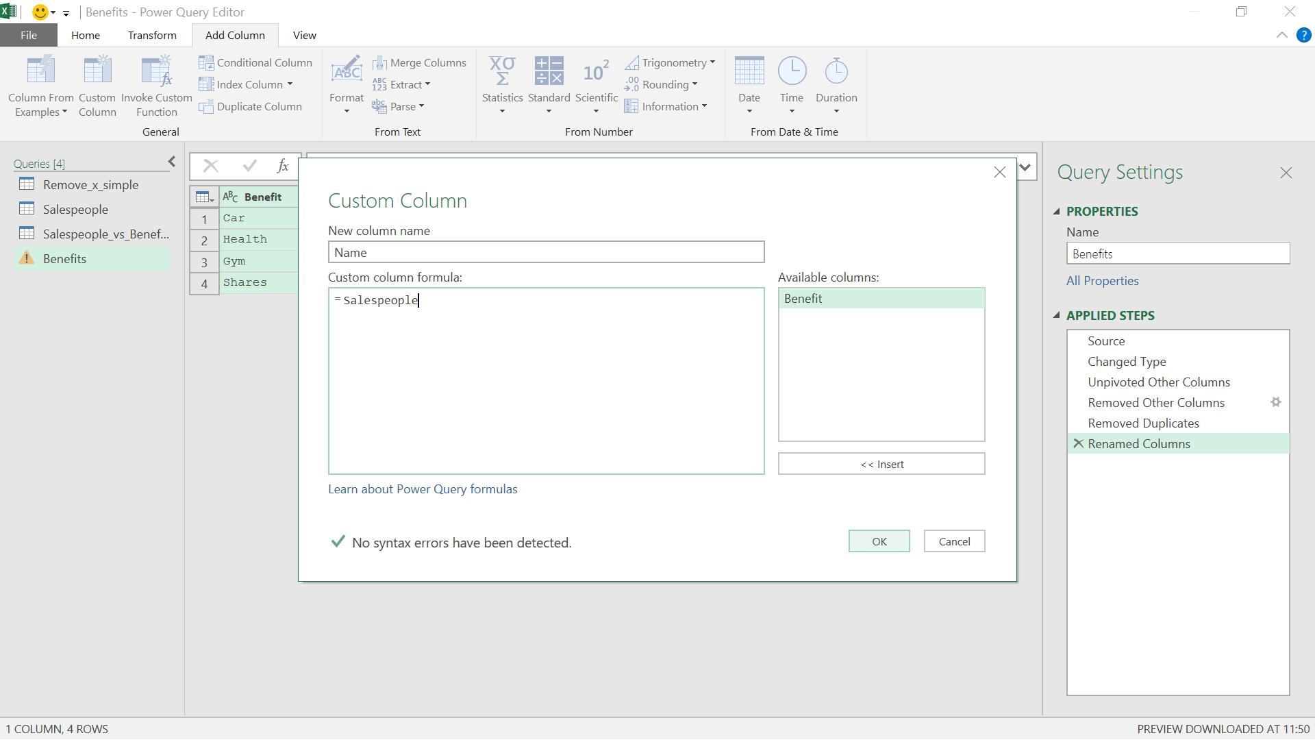
I add a ‘Custom Column’ from the ‘Add Column’ tab. I like to open the query pane to the left of the screen so that I know the names of my other queries:
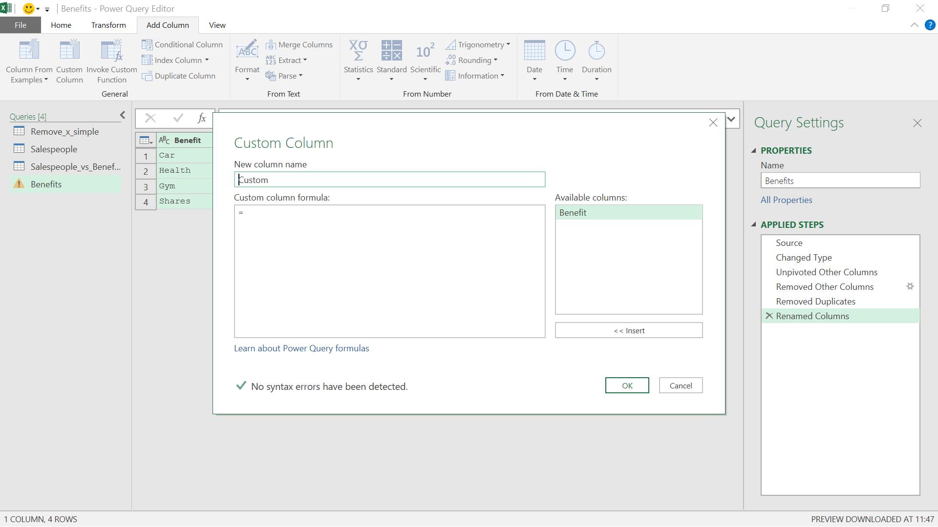
I am going to add the salespeople first, so I use the ‘Salespeople’ query:
This initially gives me a table in each row.
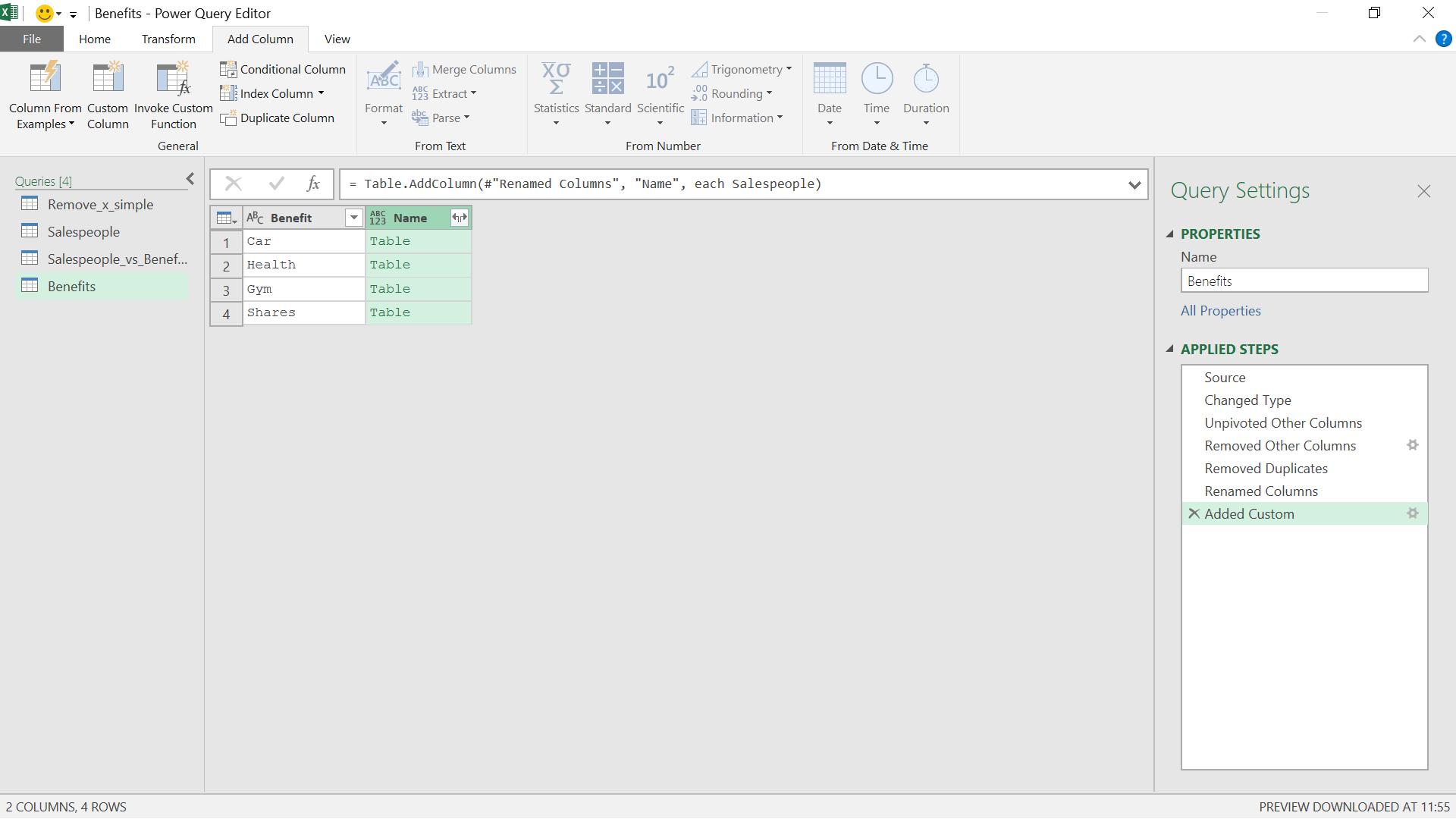
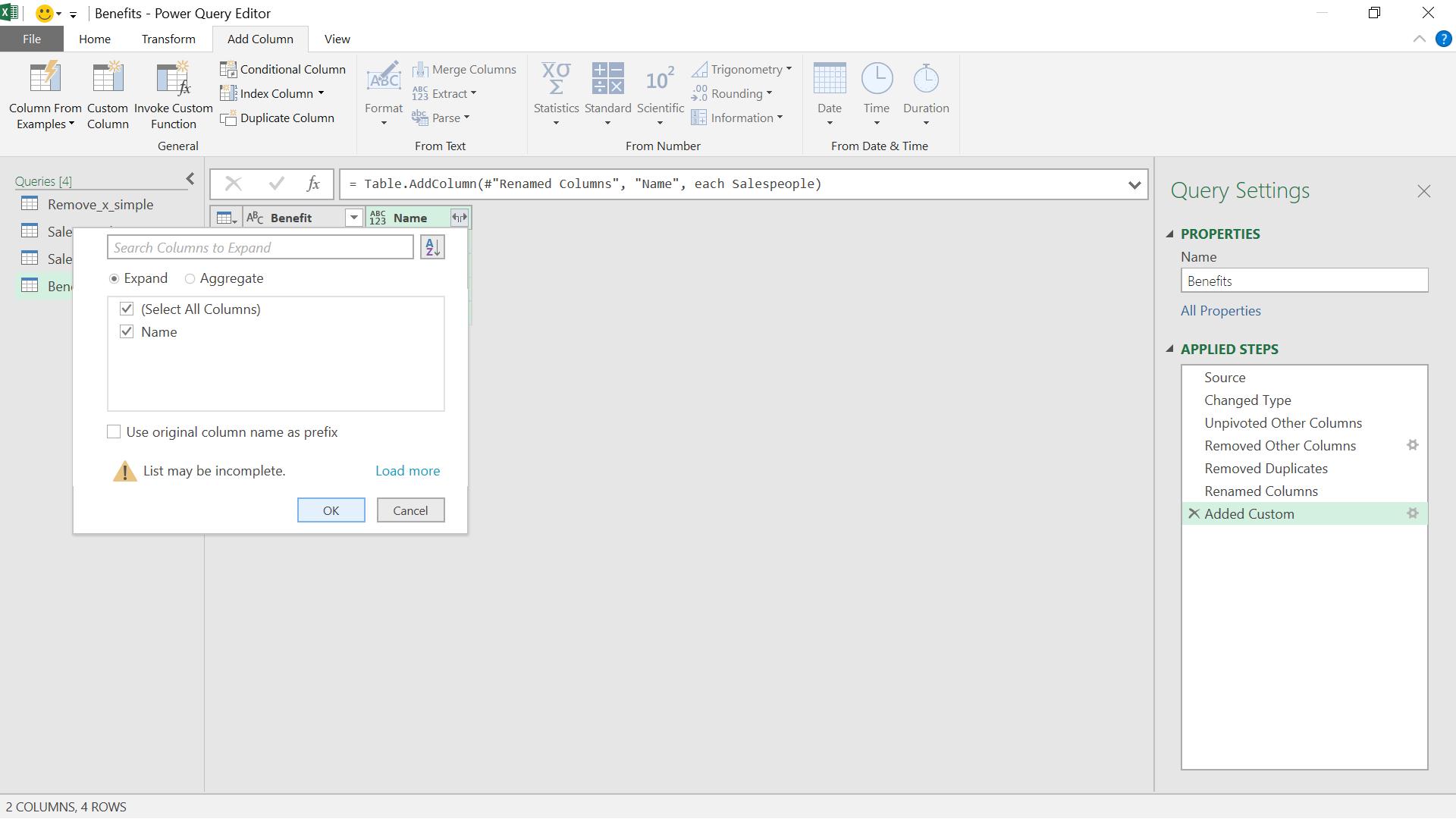
I can expand my table using the icon next to the column heading.
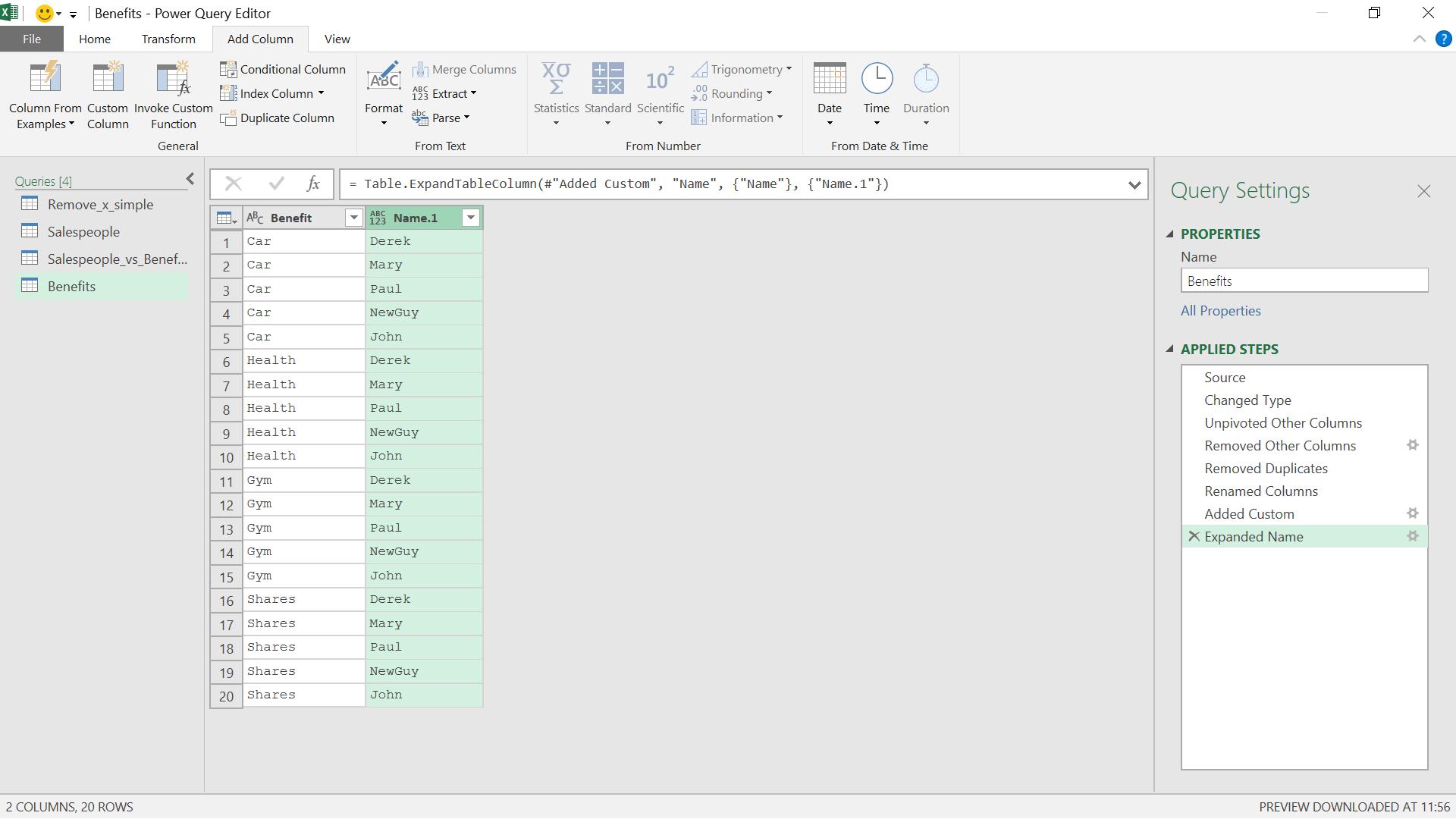
Now I’m sure the salespeople would like this (especially NewGuy), but the data now shows all the possible combinations available – I need to change this to show those that are actually received!
I start to get my data ready to resemble the table I want by putting Name first and sorting on Name.
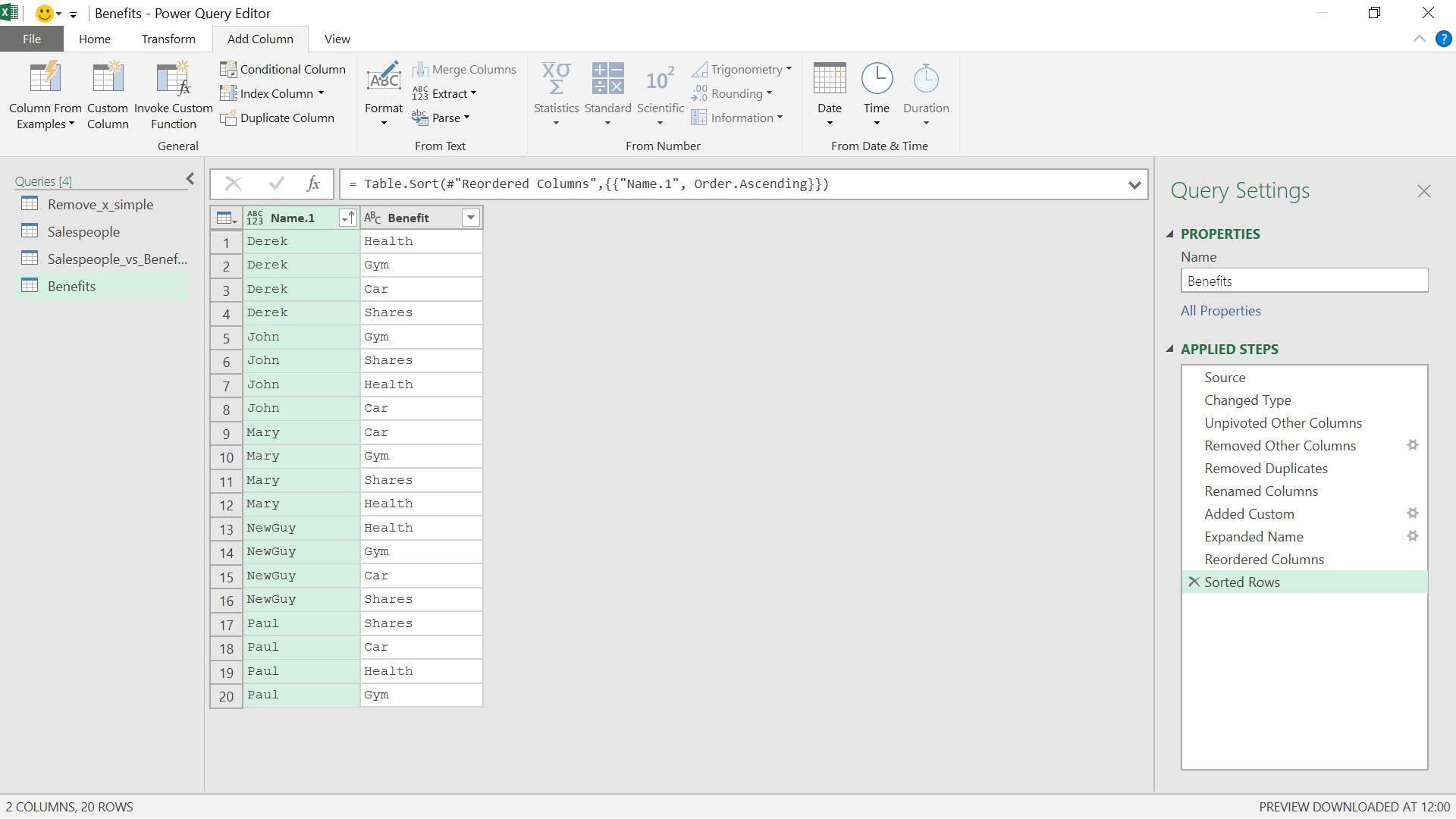
I am going to save this query as ‘Available_Benefits’, and I am going to create a new query by merging some of my existing queries.
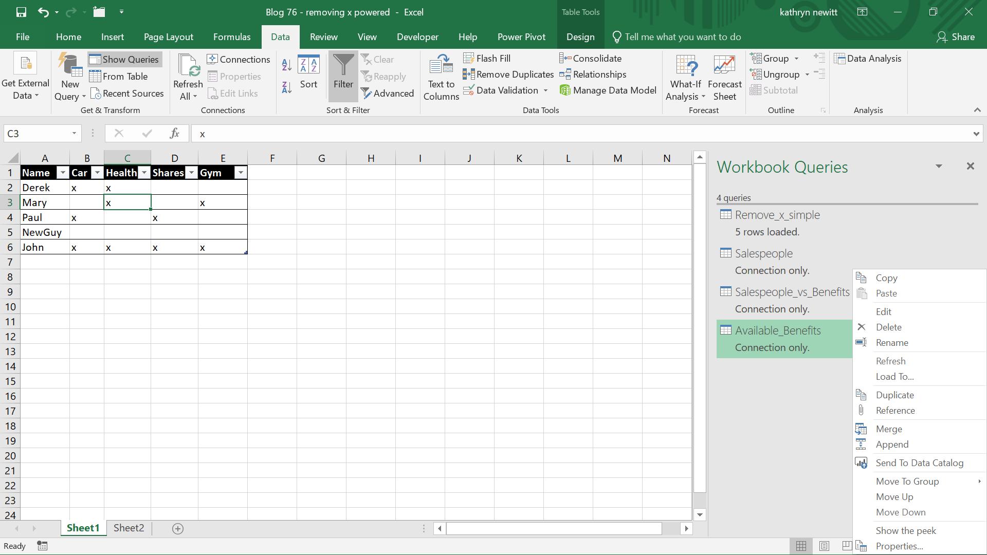
I access the ‘Merge’ option by right-clicking on the ‘Available_Benefits’ query. I want to merge ‘Available_Benefits’ with ‘Salespeople_vs_Benefits’ – linking all the possible benefits to the ones that are actually received. This will allow me to keep ‘NewGuy’, as he is in the ‘Available_Benefits’ table.
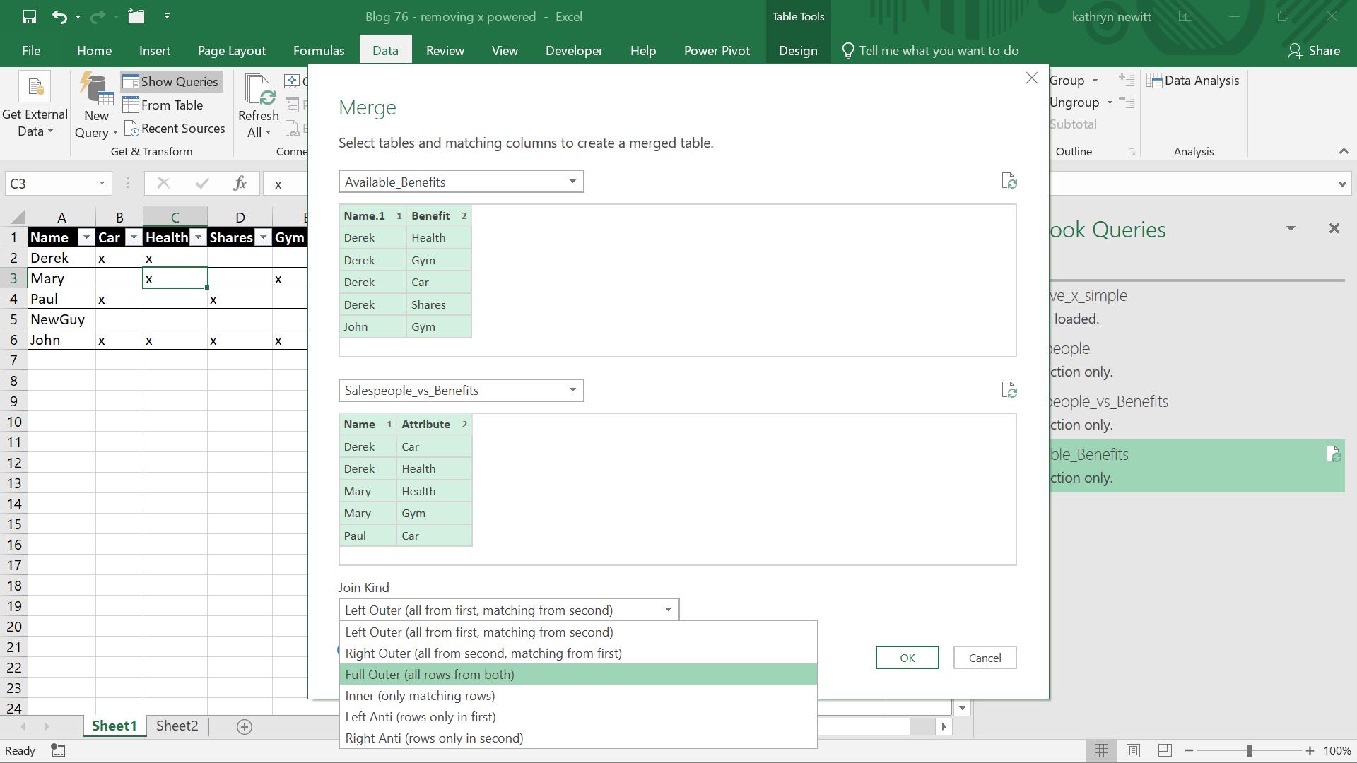
I want to join by matching both of my columns, and I need to include everyone in the first query (so that ‘NewGuy’ doesn’t get left behind) and all the data in my second query (as that tells me who gets the benefits). I choose a ‘Full Outer’ join (you can read more on this in Power Query: If You Can’t Tell Them Apart, Join Them).
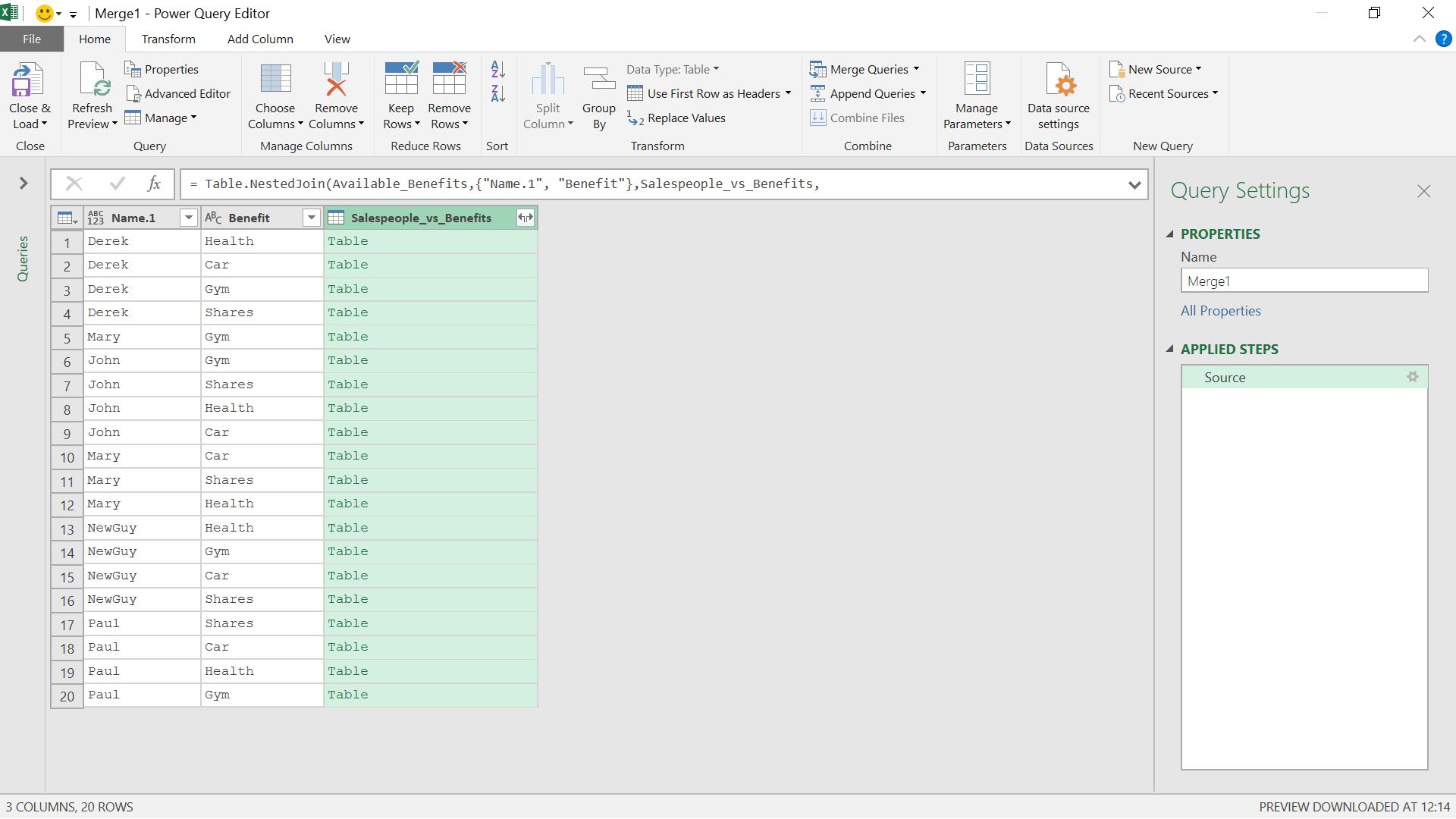
I can expand the Salespeople_vs_Benefits column to show all the columns in that table.
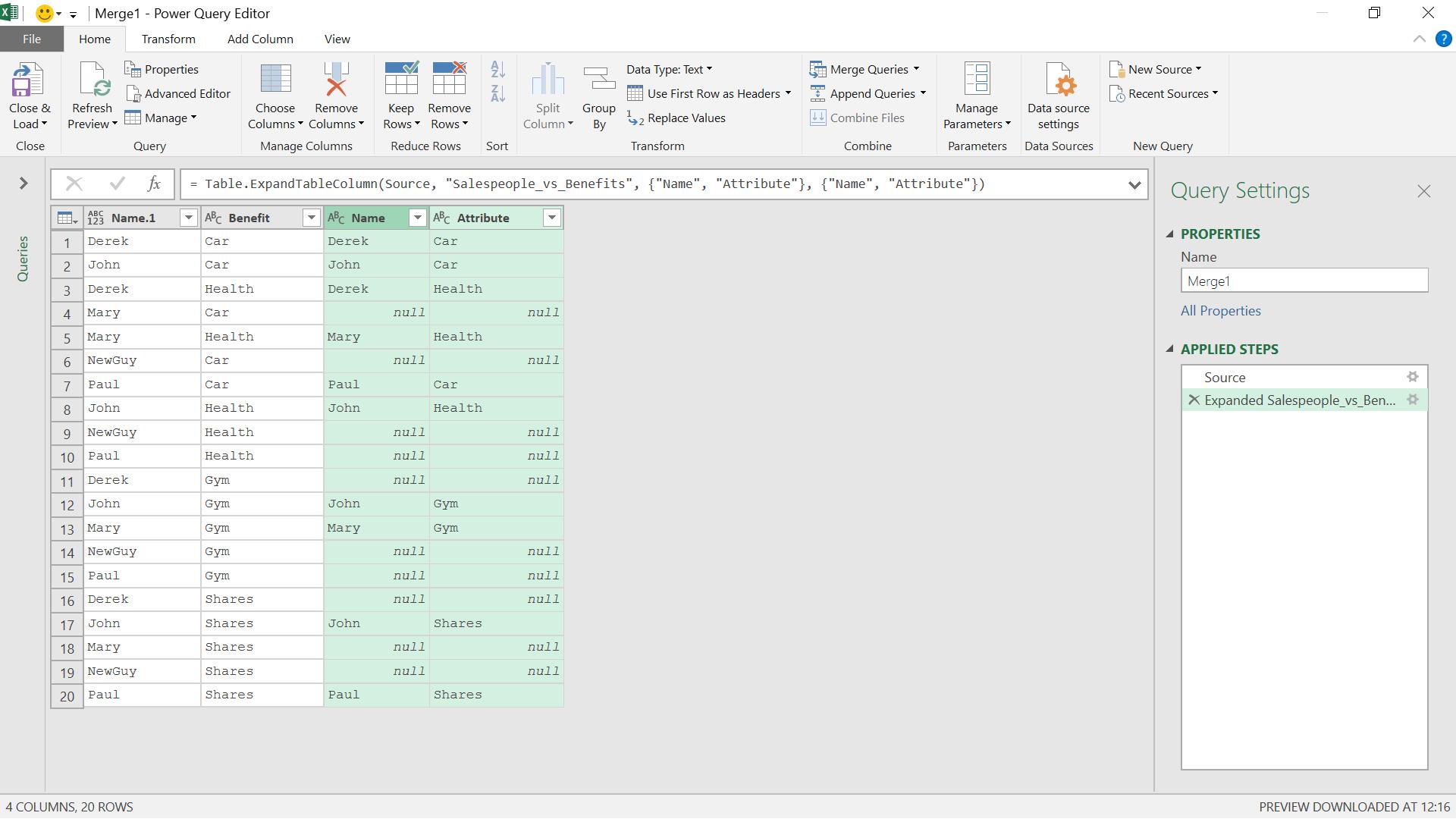
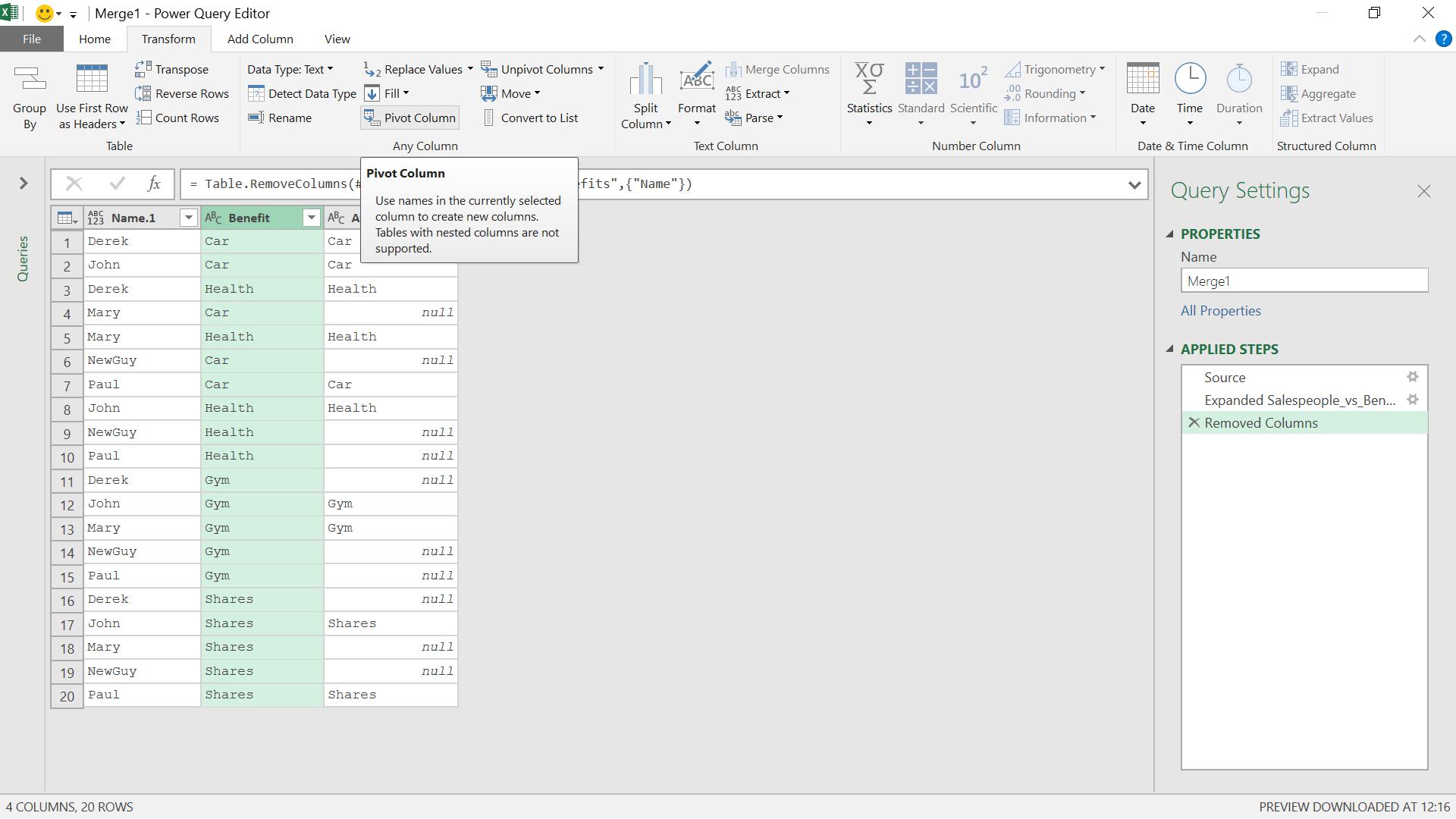
Now I can see that I am starting to get the data in the format I would like. I just need to get rid of the Name column and pivot the Benefit column so that it becomes the headings. I can do this by selecting the Benefit column and choosing the ‘Pivot’ option in the ‘Any Column’ section on the ‘Transform’ tab.
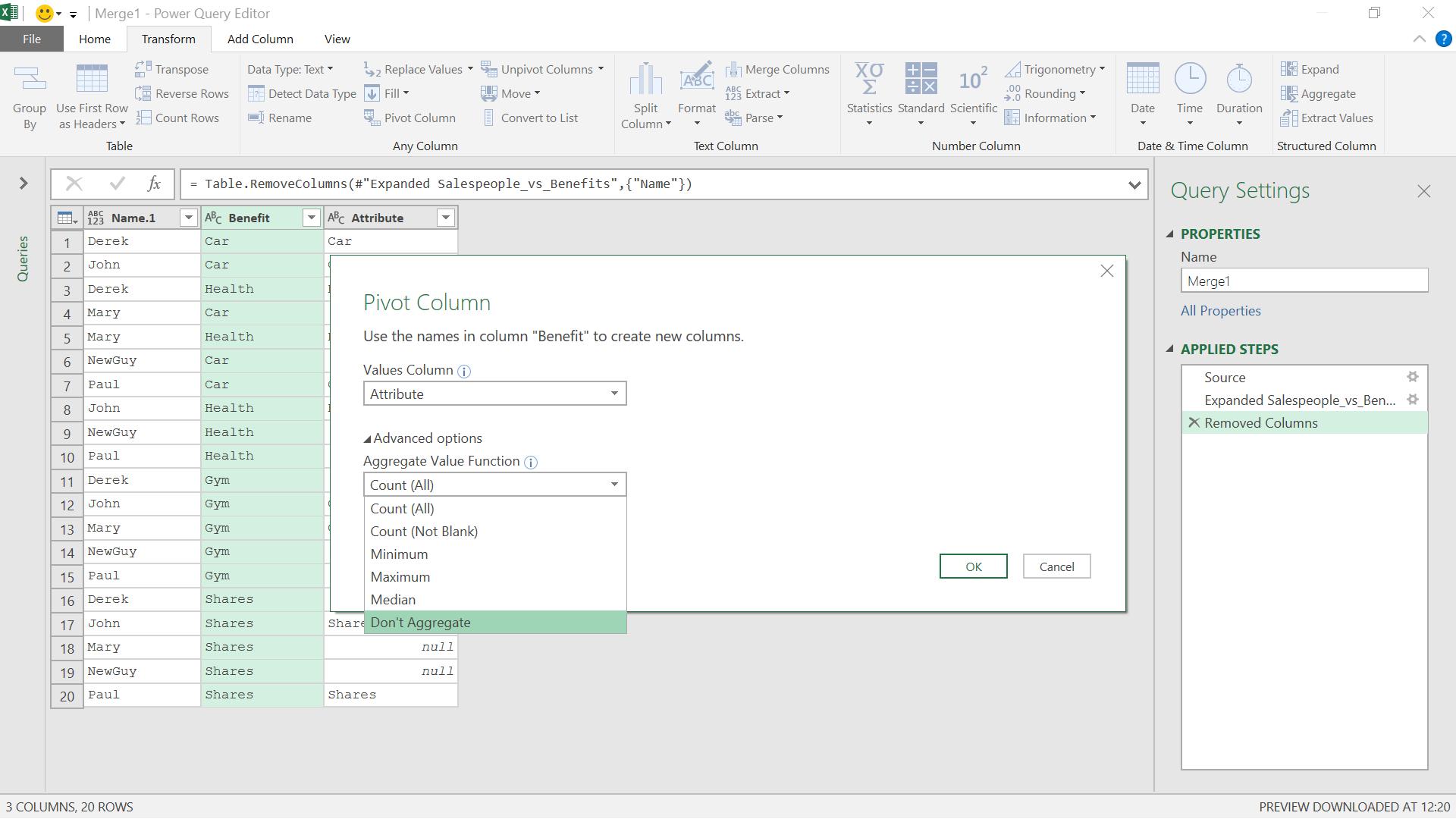
The values need to come from the Attributes column, as that holds the logic for the benefits, and I don’t want Power Query to apply any aggregation.
My results are now looking good!
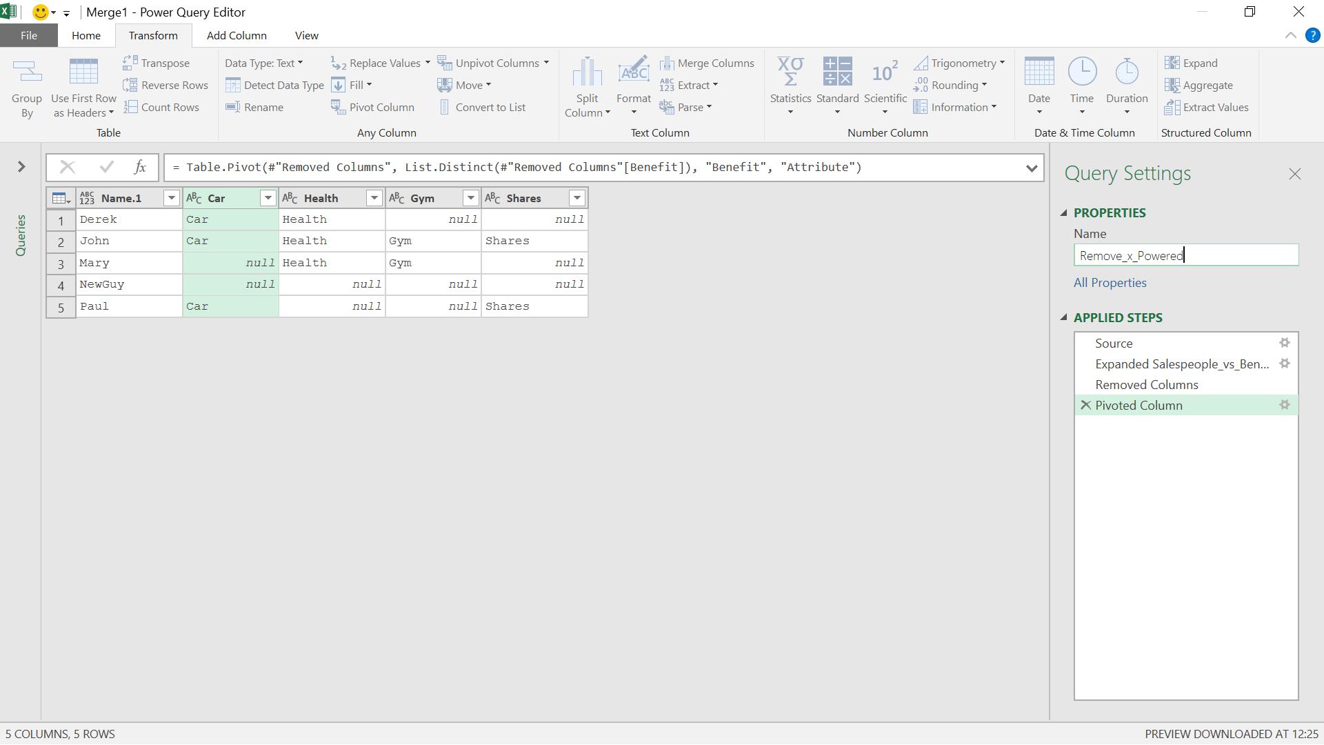
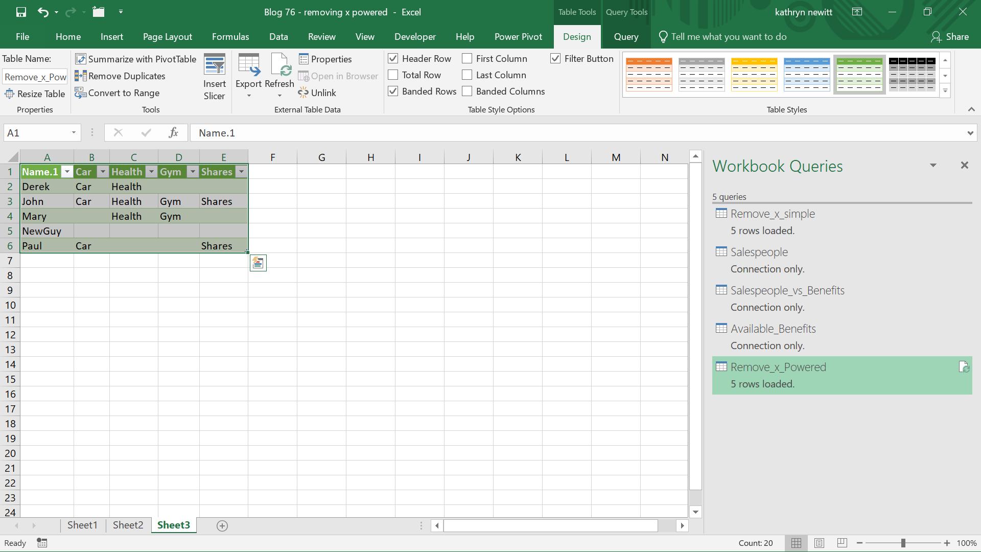
I can load this data to my worksheet:
Finally, I want to see what happens if I add a new benefit and refresh my query.
A new bonus scheme has arrived, but not everyone is eligible! I refresh my query.
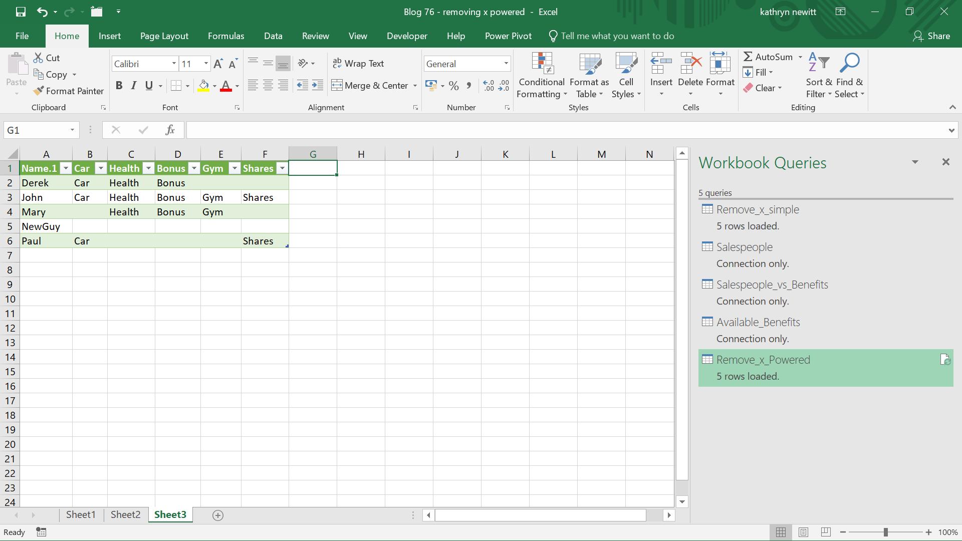
Derek, John and Mary are clearly on the bonus scheme. As I have broken the query down and reconstructed it, any changes to benefits or staff will be reflected when refreshed.
Come back next time for more ways to use Power Query!