
Power Query: The Delete Dilemma
22 July 2020
Welcome to our Power Query blog. This week. I look at data from a sheet made up of a number of tables, with a random amount of data that needs to be excluded.
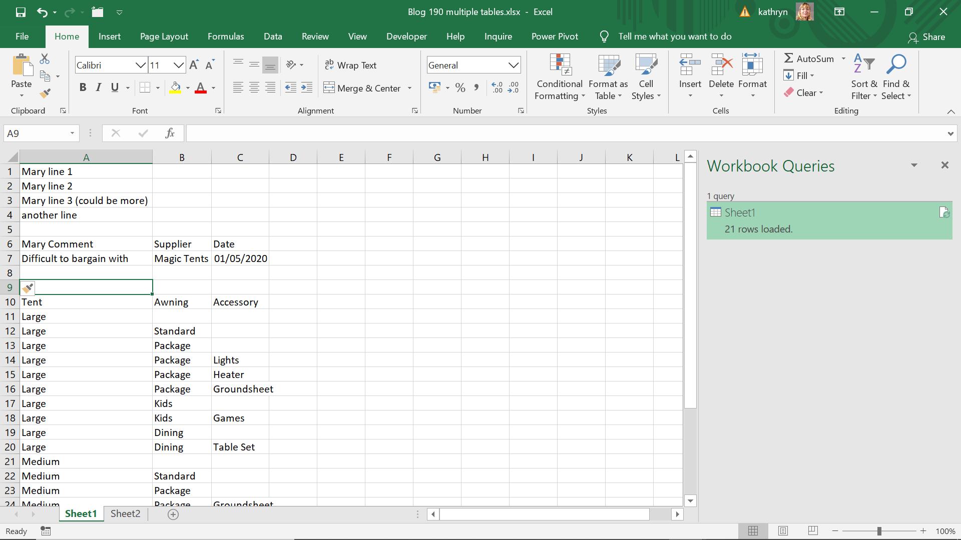
Mary, one of my imaginary salespeople, has sent in a slightly unusual report of the tents available from a particular supplier.
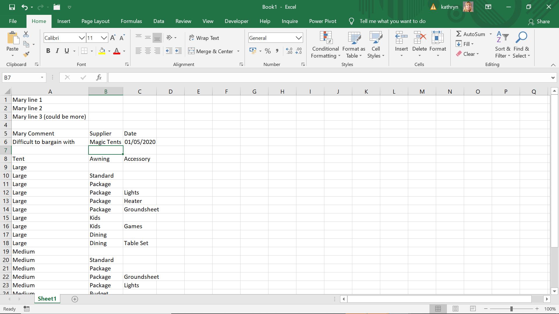
I want to put the tent, supplier and report date into a table, and delete the lines at the top (there will be an unknown number of these). I begin by extracting my data to Power Query, using ‘From Table’ on the ‘Get & Transform’ section of the Data tab.
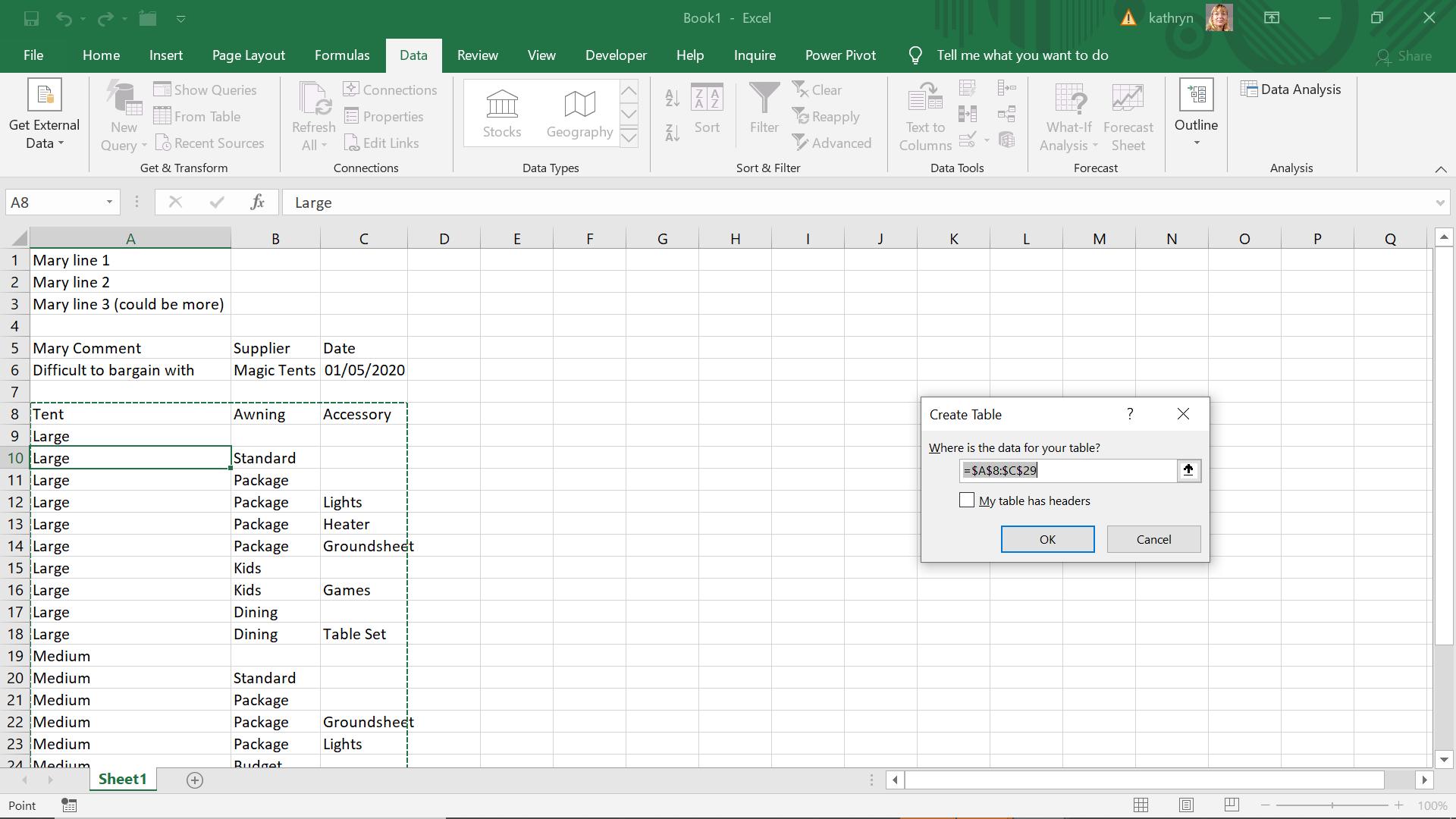
The ‘Create Table’ dialog box tries to default to the table I happen to be in, but I need to change this to include all of my data; instead of using ‘From Table’, I will adopt another approach.
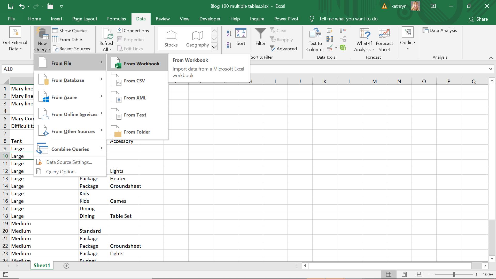
I select ‘From Workbook’ in the dropdown from the ‘From File’ option on the ‘New Query’ options, and select my current workbook.

I select the sheet.
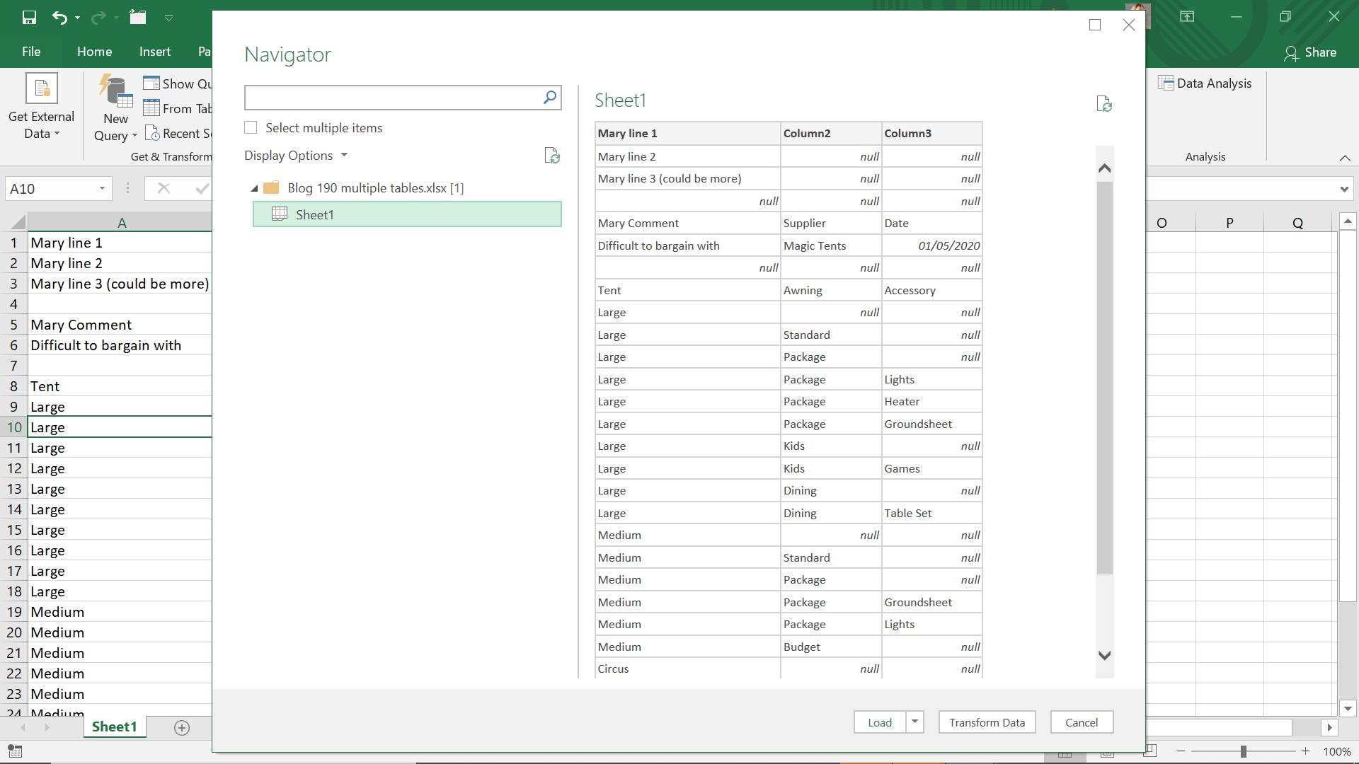
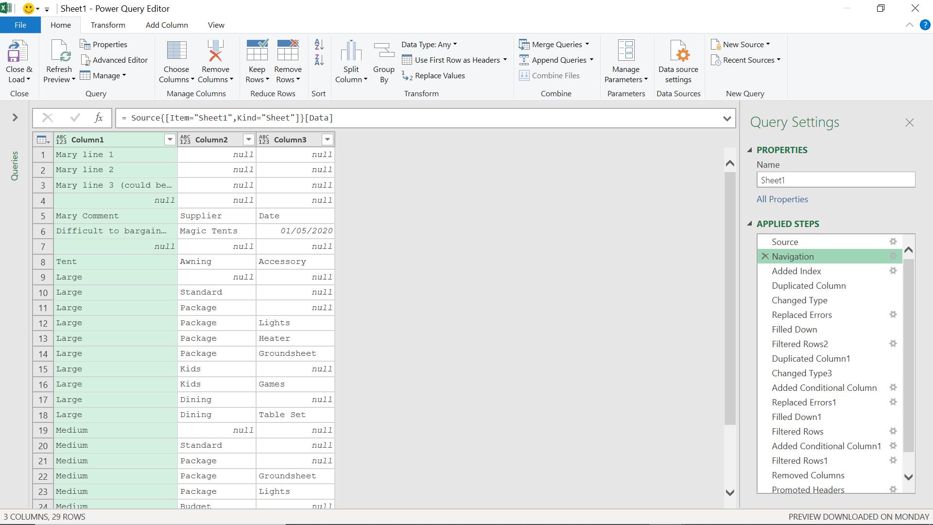
I can see that all my data has been included; I can now choose to ‘Transform Data’.
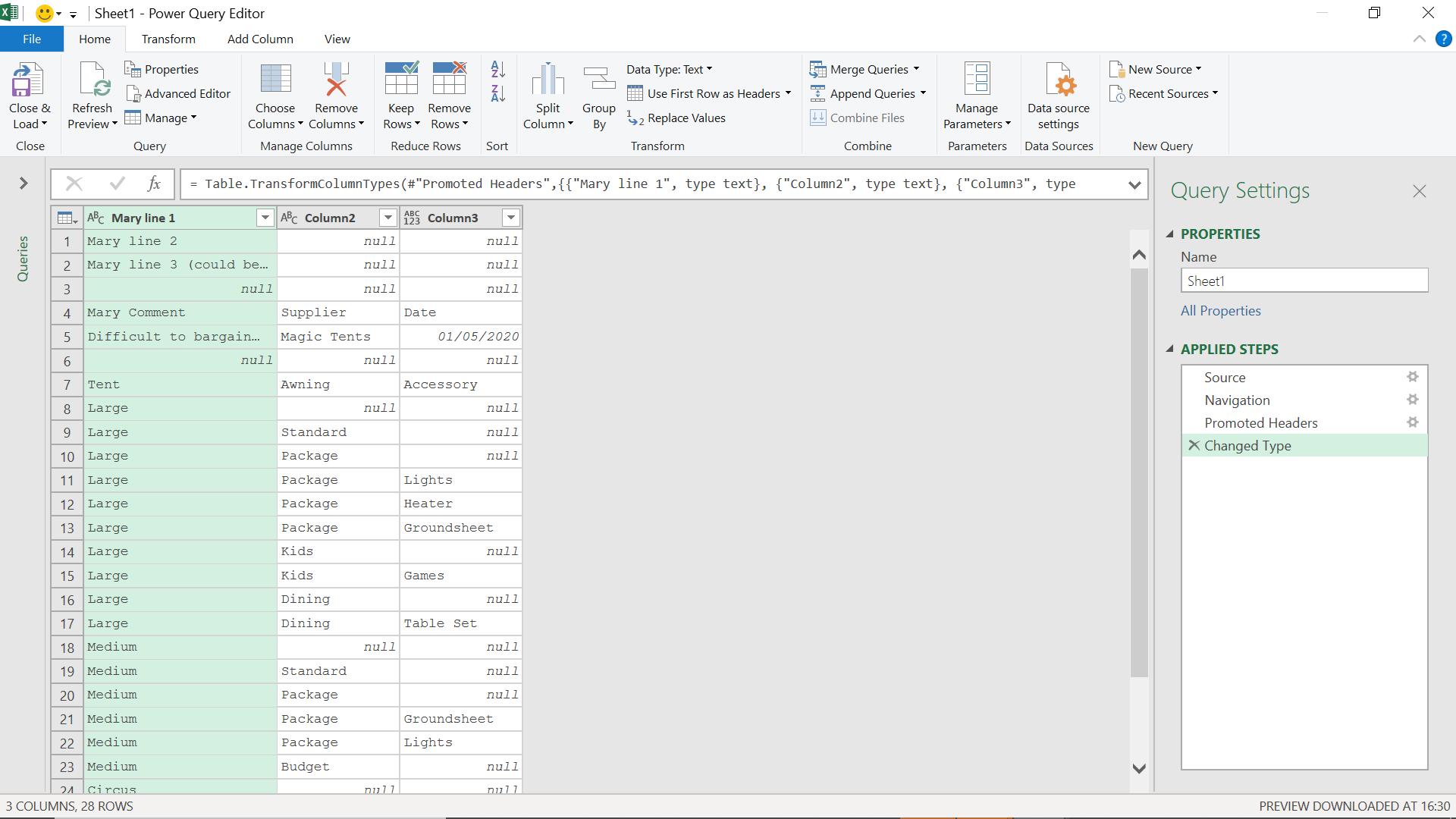
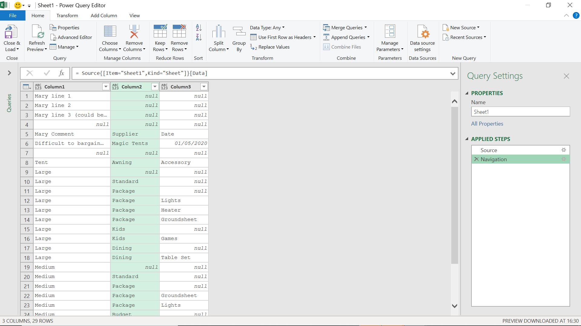
Power Query has automated some steps, but I don’t want to include most of them, so I delete all steps after the ‘Navigation’ step.
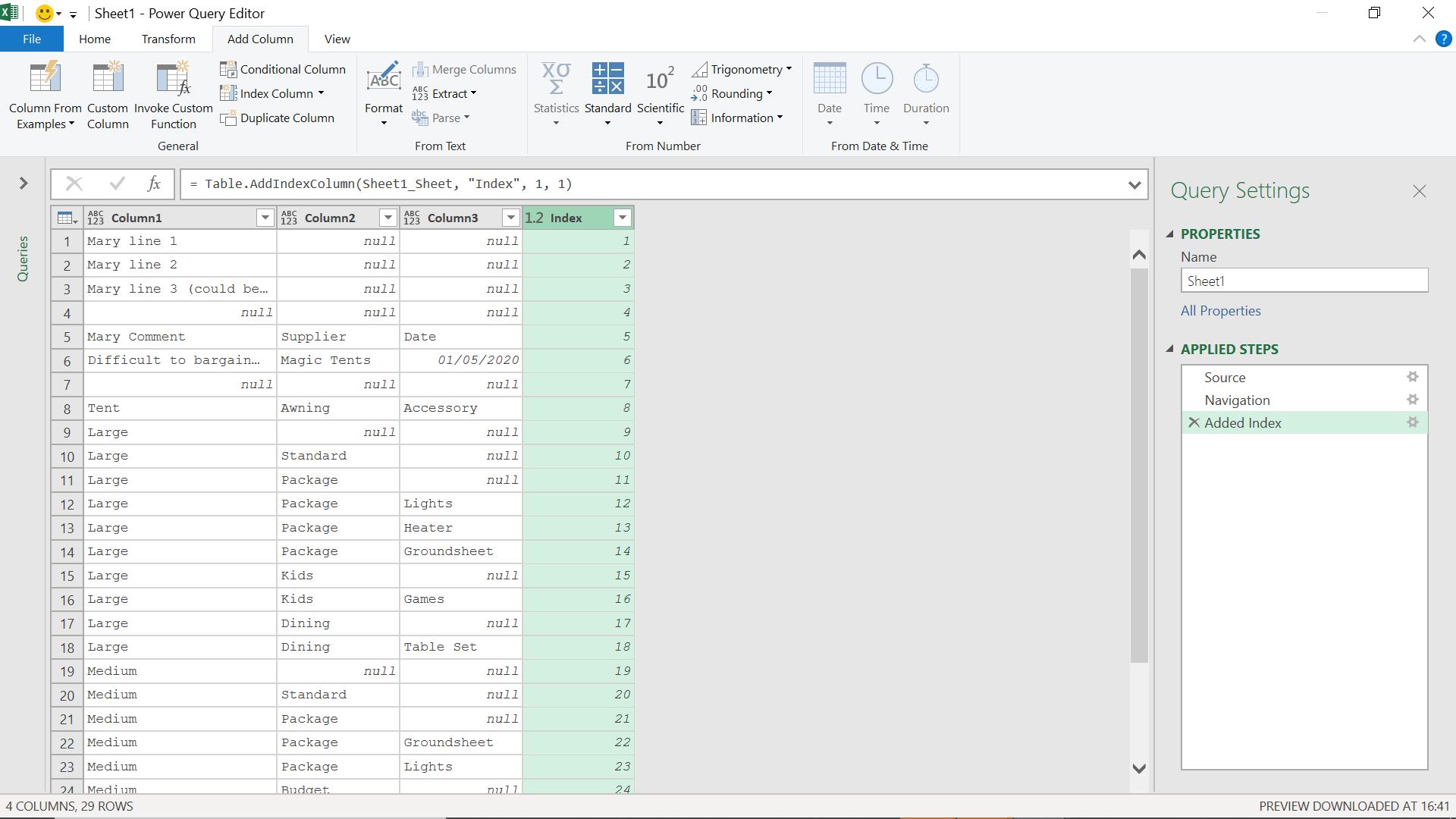
I need to remove the top rows, but I want to avoid specifying how many of these rows there are. I plan to delete all rows above the date value. I begin by adding an index from the ‘Add Column’ tab.
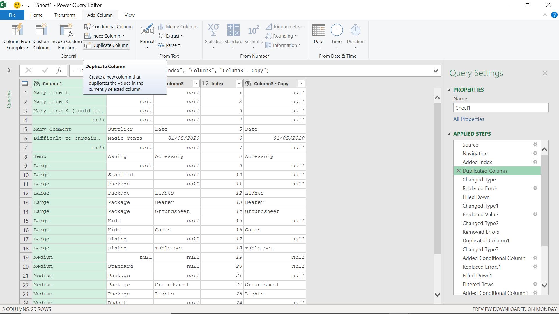
Next, I create a duplicate column of Column3 (which contains the report date value) on the ‘Add Column’ tab.
In order to get rid of all the data apart from the date, I convert Column3 – Copy to Data Type ‘Date’. This may be done from the ‘Transform’ tab.
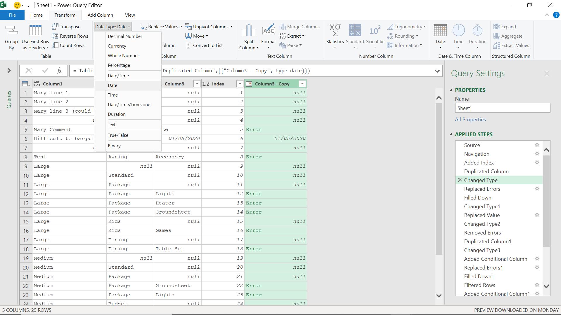
This means that apart from the date, the data values are now either null or Error. If I right-click my column, I can replace the errors with null values.
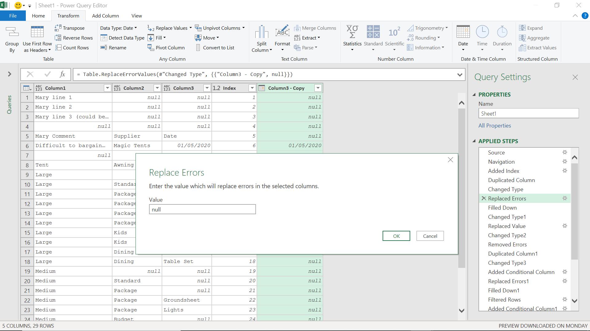
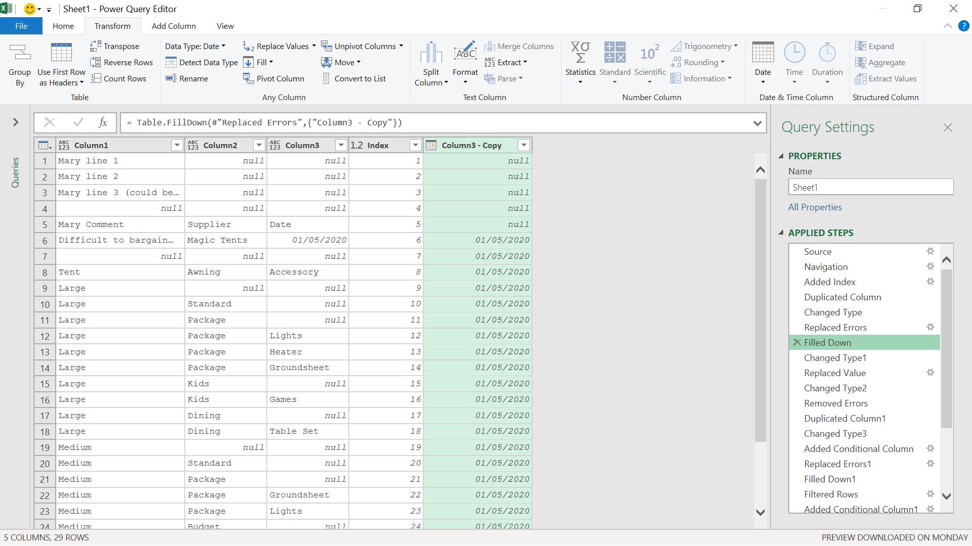
This gives me null values, and I can now fill down by right-clicking, choosing to ‘Fill’ and then choosing to ‘Fill Down’. The rows above the date do not matter as I want to delete them.
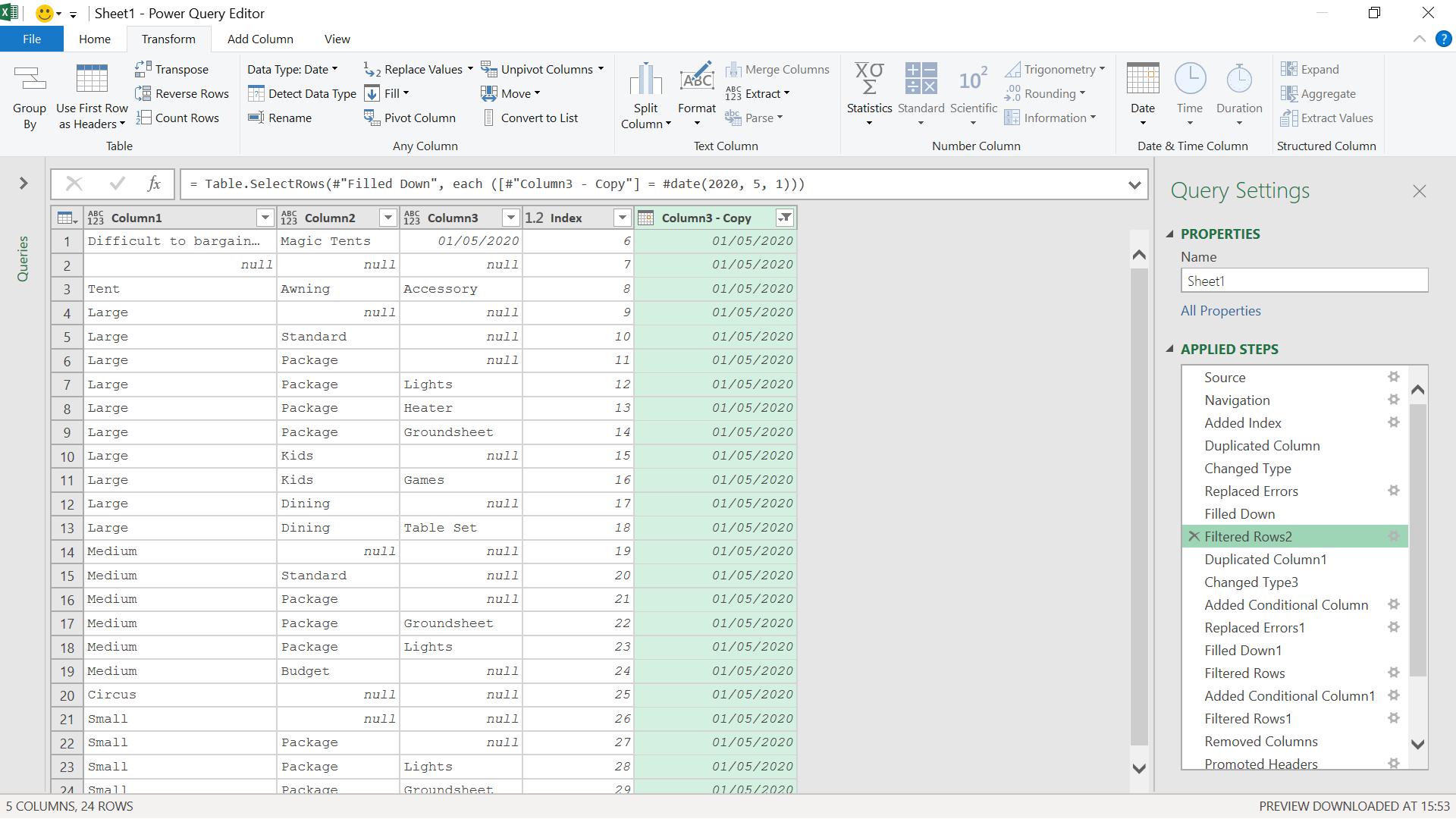
I need to delete the null value rows, so I filter and choose values that are not null.
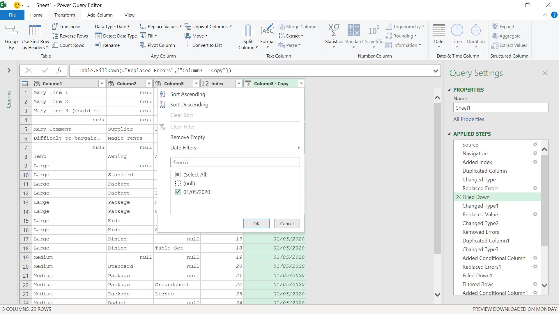
This gives me the rows with a date value.
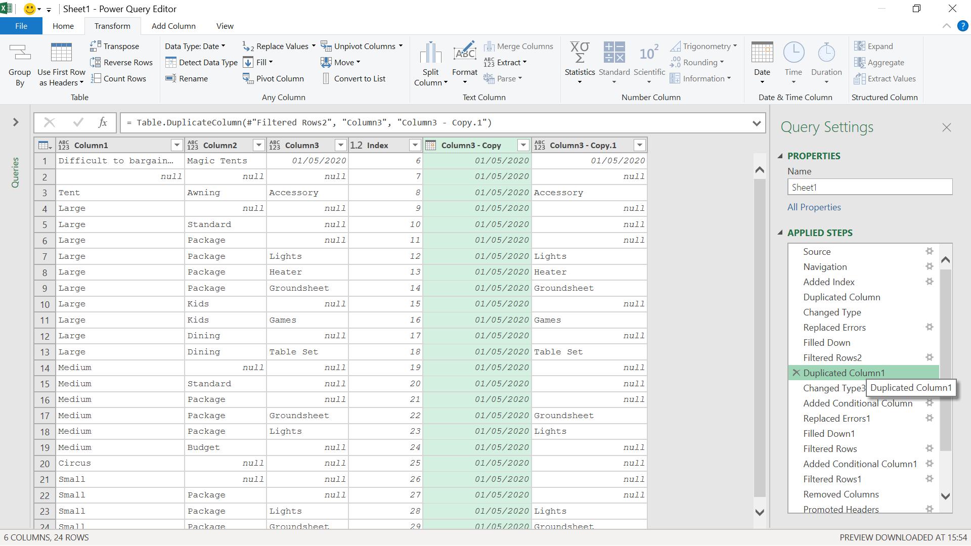
I have the date column. Now, I want to get the supplier into a column. I create another duplicate of Column3:
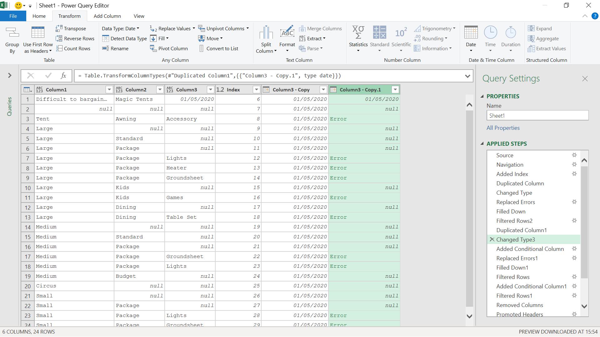
I convert the Data Type on my new column to ‘Date’ because I want to isolate the value with the date.
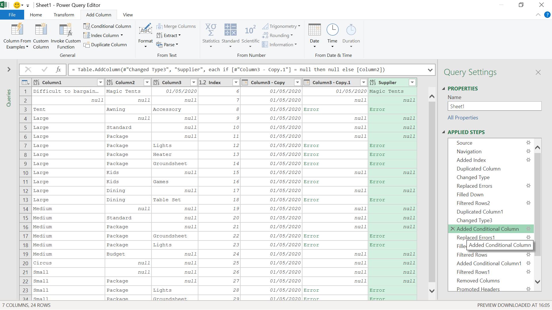
I create a new conditional column from the ‘Add Column’ tab.
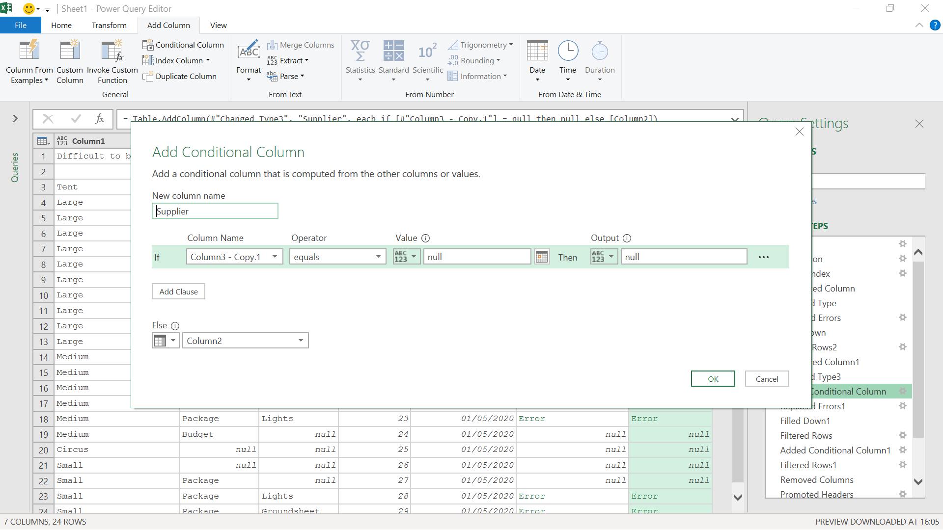
If the value is not null, then I want to put the supplier from Column2 into my new column, which I call Supplier. The values with errors will remain as errors.
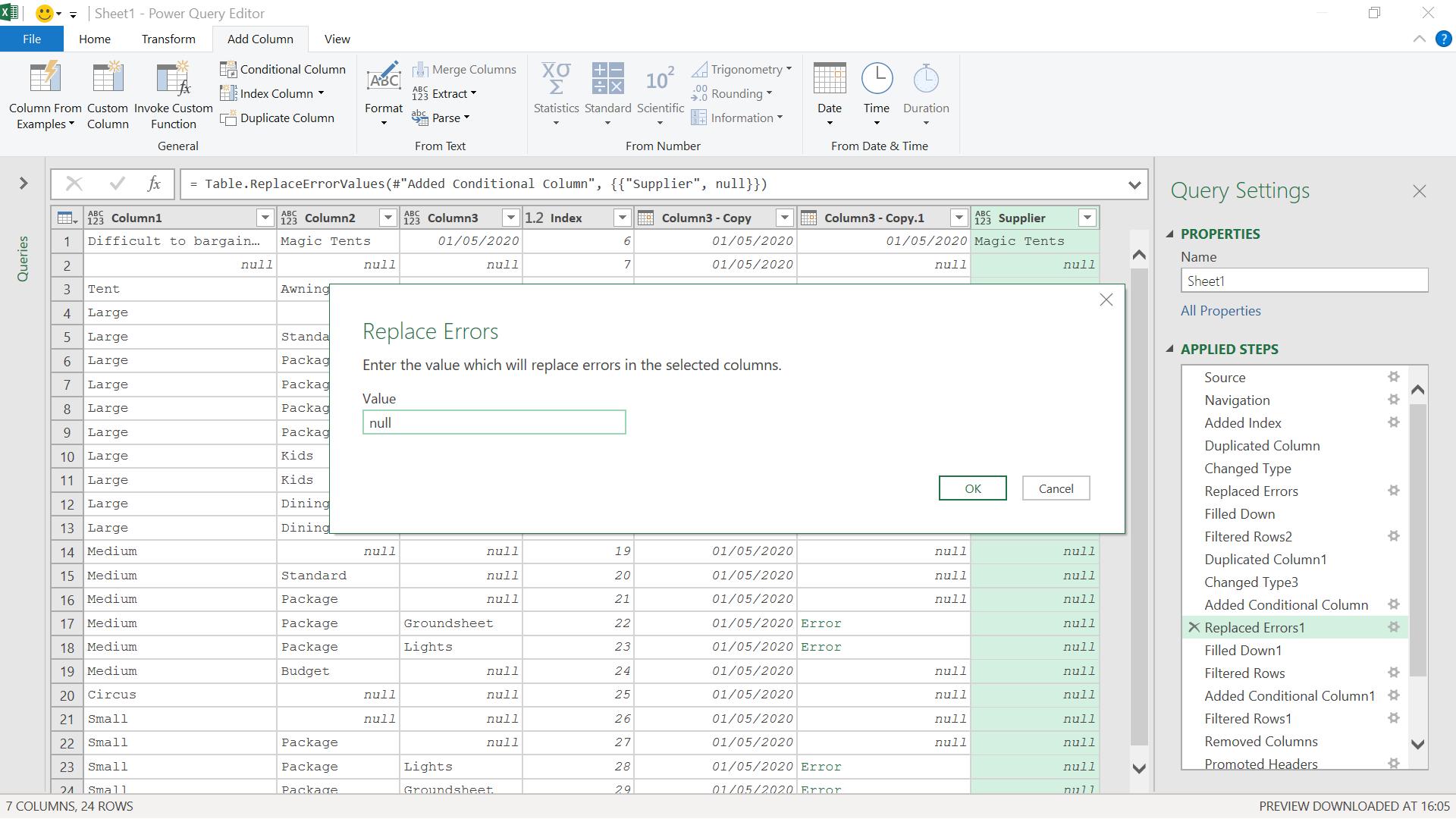
I can now right-click on Supplier and replace the errors with null.
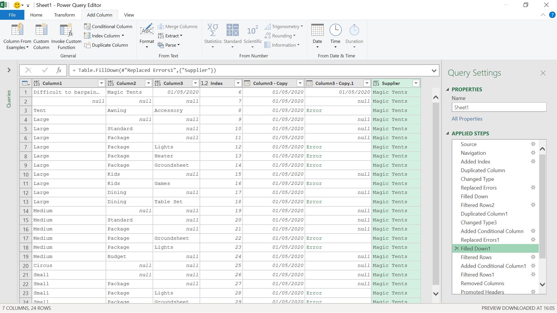
Having done this, I can fill down my supplier, as before.
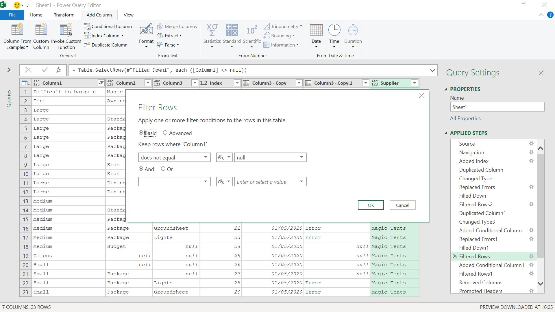
I have one more row to remove, and I can do this by filtering on Column1 to remove null values.
I have one final row to delete, but this time it has values in all columns.
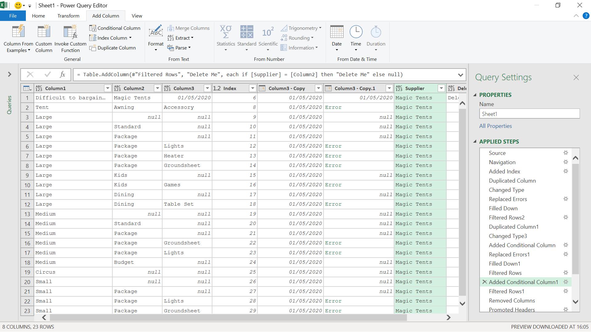
The data I need in the top row has already been moved to columns. I could just delete the top row, but instead I choose to identify it by creating a new conditional column.
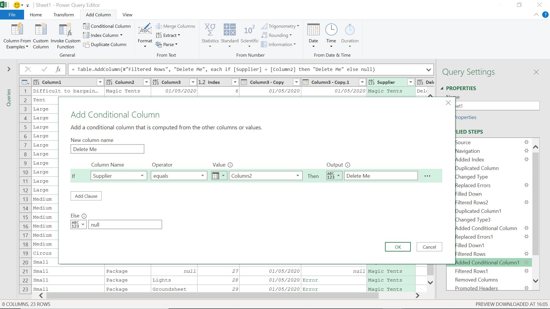
I choose to create a new column which will indicate a row should be deleted if the value in Supplier matches the value in Column2.
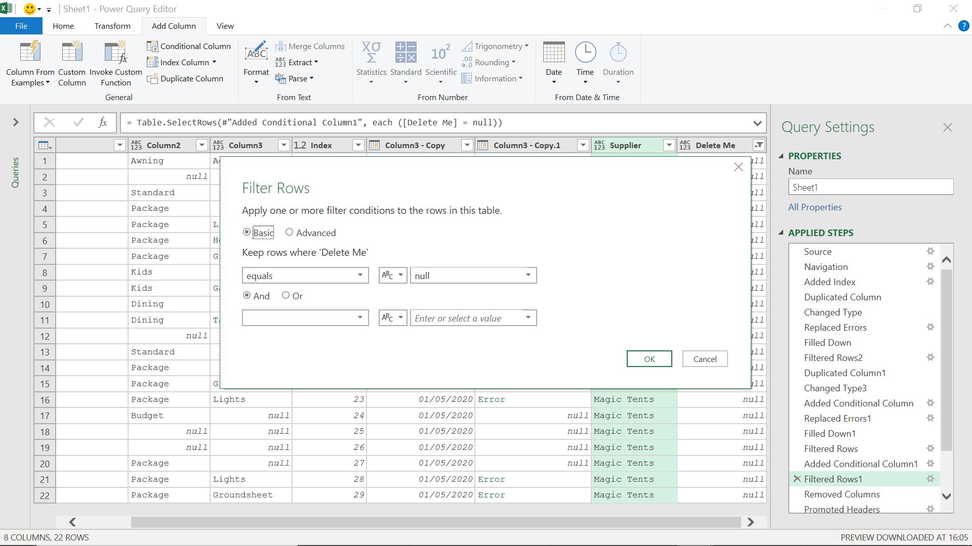
I can then filter the Delete Me column to remove everything that isn’t null.
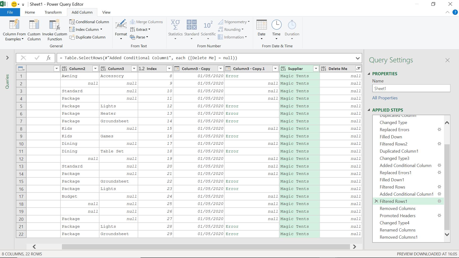
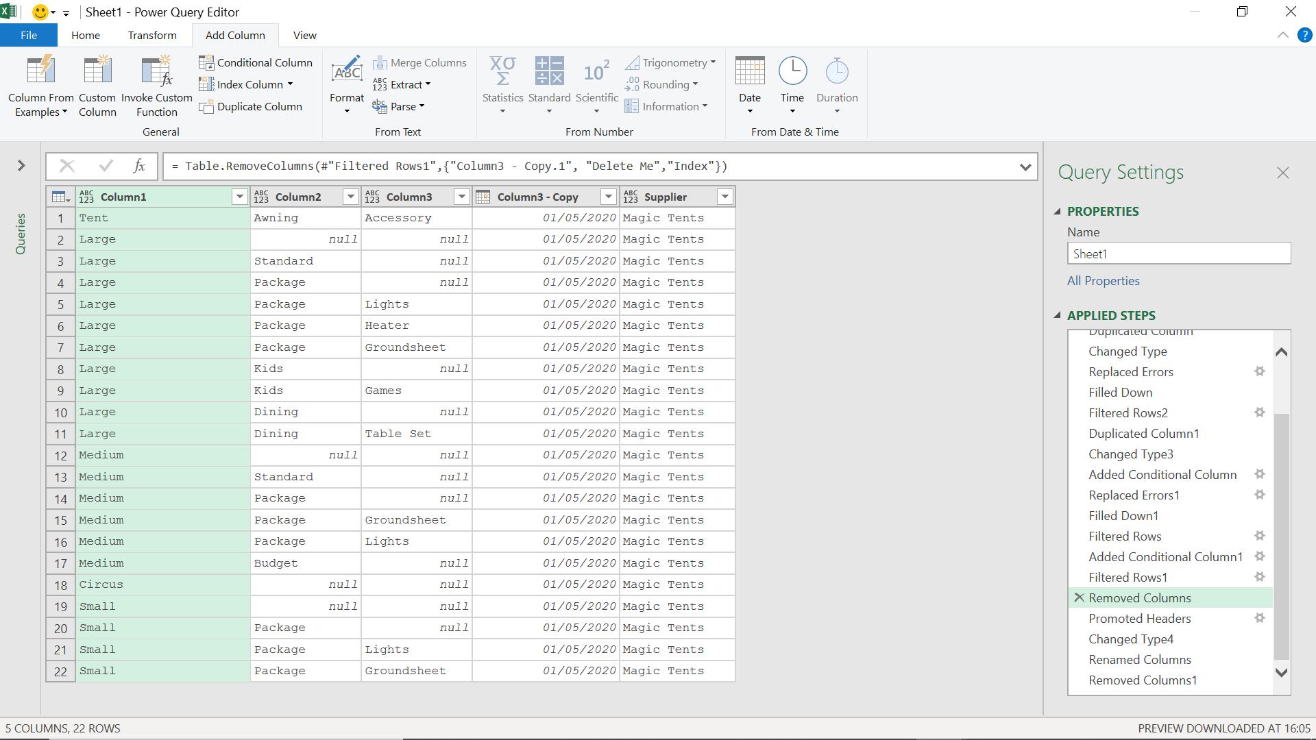
I now consider the column headings, but first I want to remove Column3 – Copy1 because the errors might cause problems. I also remove my other temporary columns at the same time.
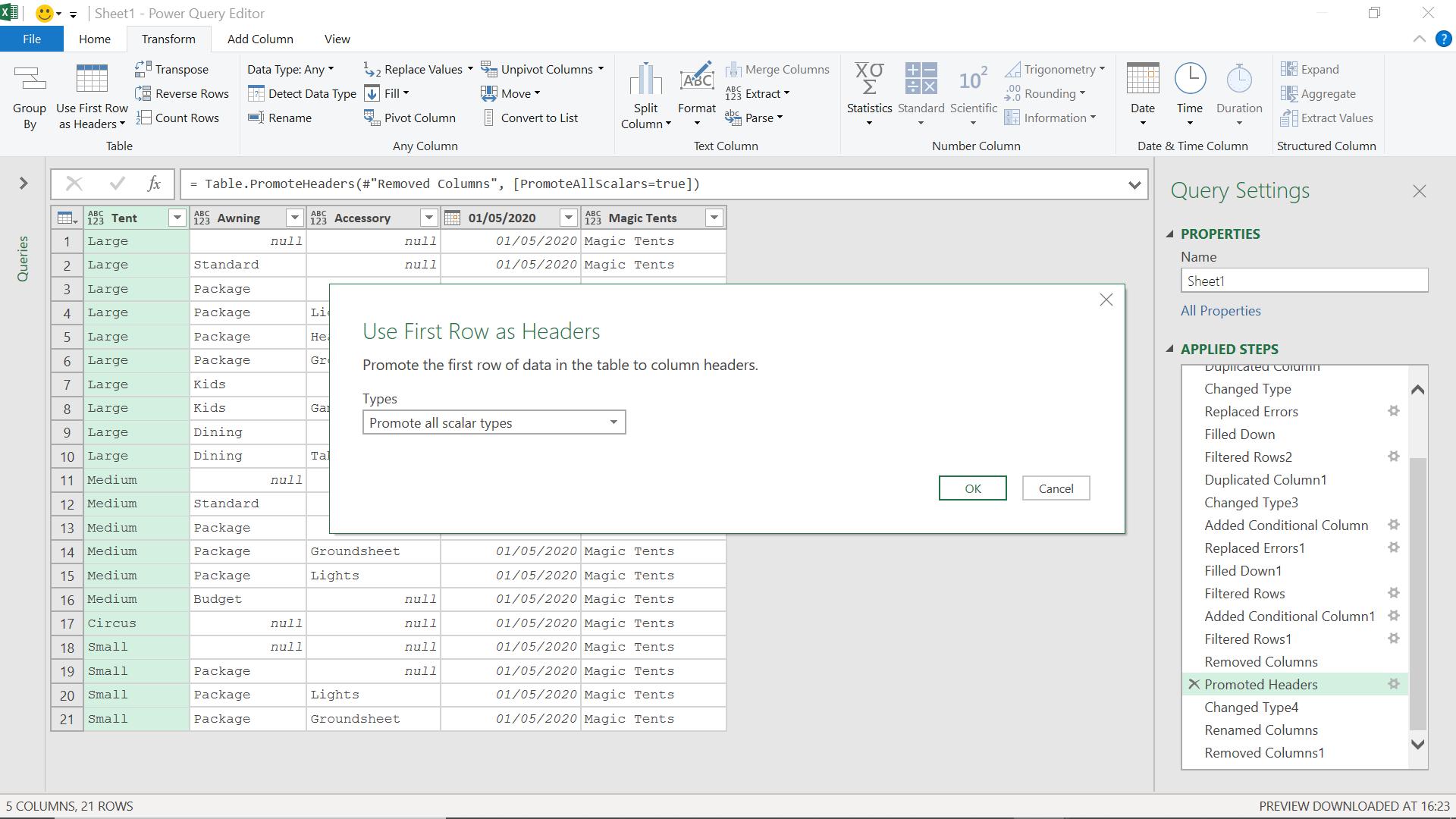
I can now promote the first row to headers from the Transform tab.
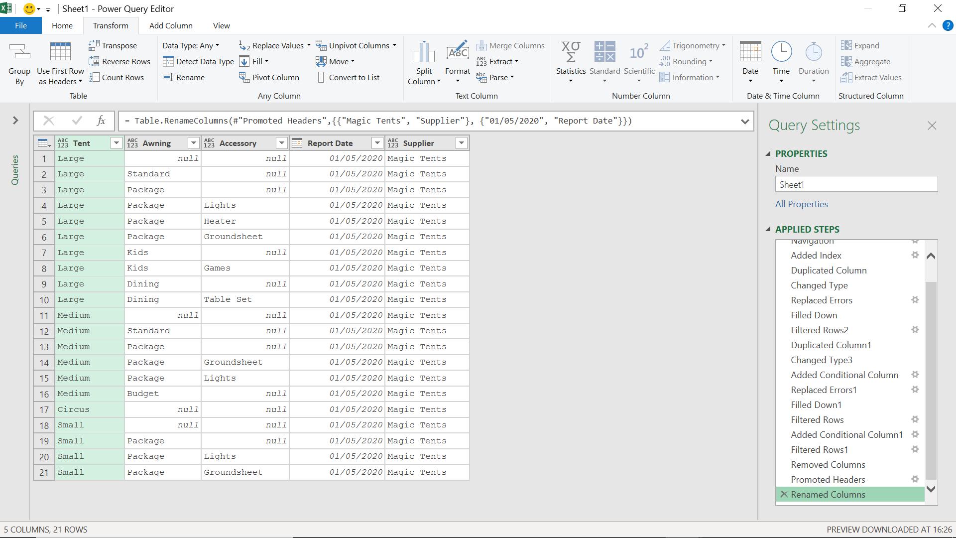
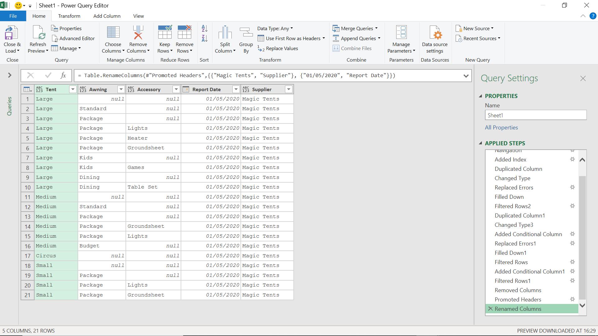
I just need to tweak the supplier and date headings.
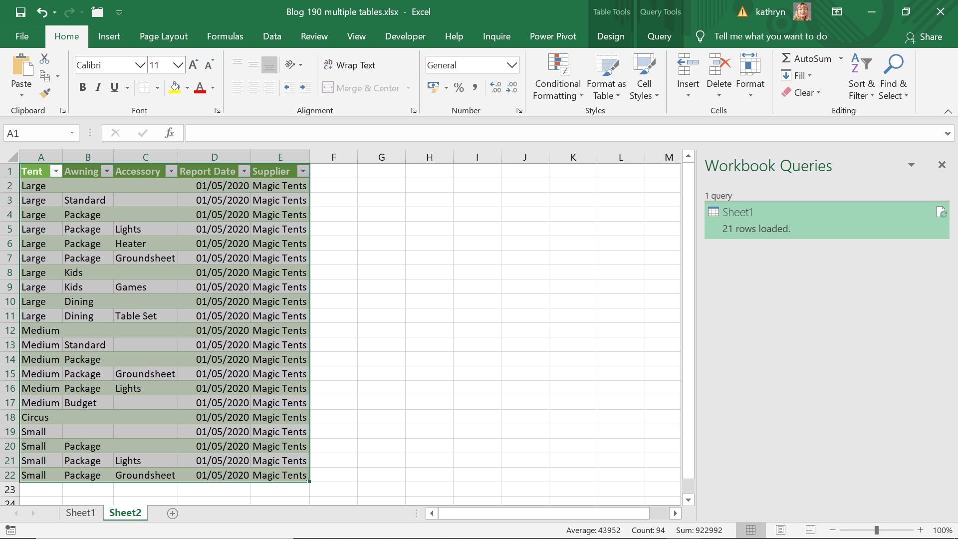
My final step is to ‘Close & Load’ my data into Excel.
If I go back and alter the data by adding some extra rows to be deleted, I can check my transformation.
I create another line at the top and an extra space before the tent data. Then, I refresh the query.
The extra lines appear in the source.
The data is still transformed correctly.
Come back next time for more ways to use Power Query!