
Power Query: Splitting Up is Not so Hard to Do
5 July 2017
Welcome to our Power Query blog. Today I look at dividing a full name column into first and last names.
This is a fairly common scenario. I have a column which is made up of several pieces of data I want to extract, in this case a full name. As a programmer, I used to write chunks of code to do this, carefully stepping through the name until I reached the space. With Power Query, it’s much easier.
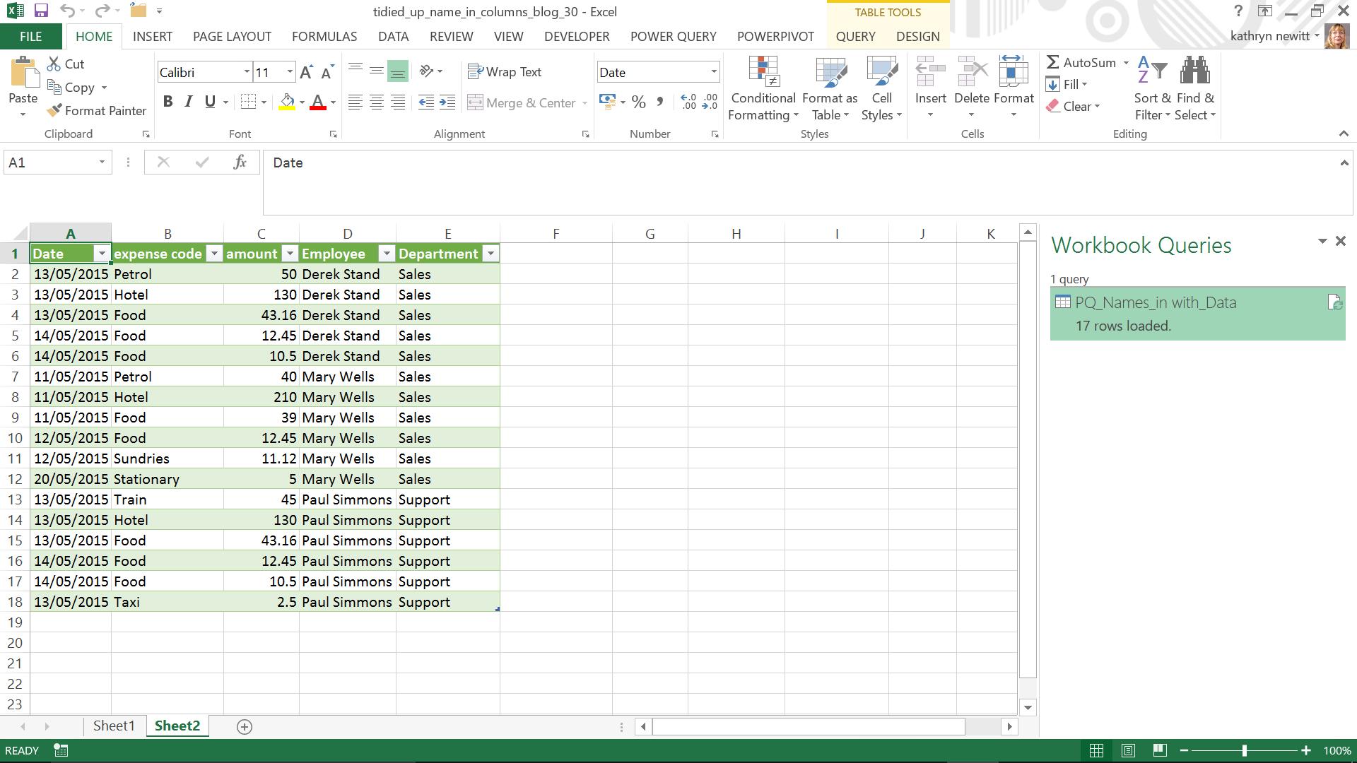
I will start from where I ended last week, with a file of expense data, which happens to include the full name of the employees. In order to show how this can be applied to any Excel data, I will load only the name to a query for this example.
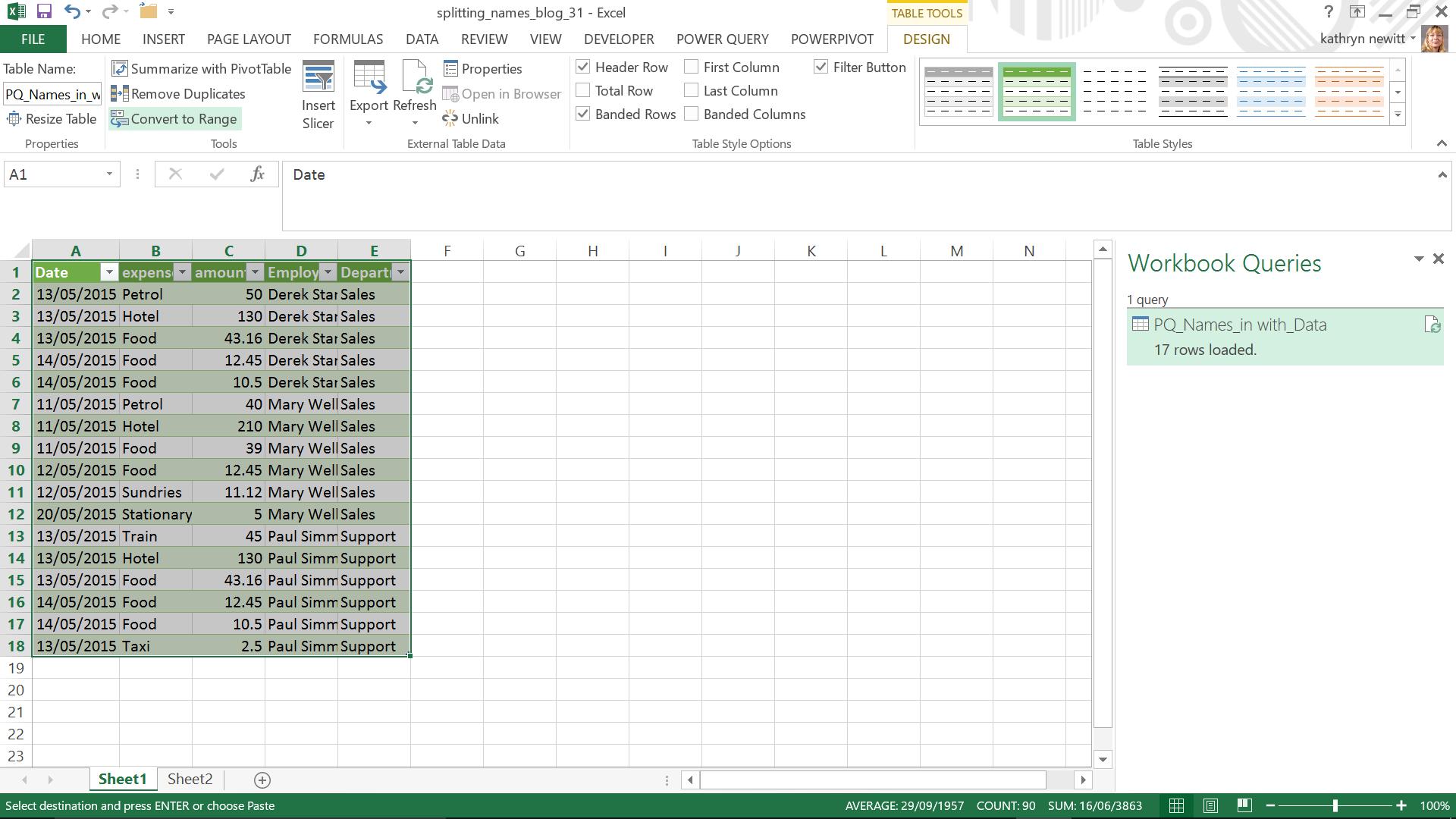
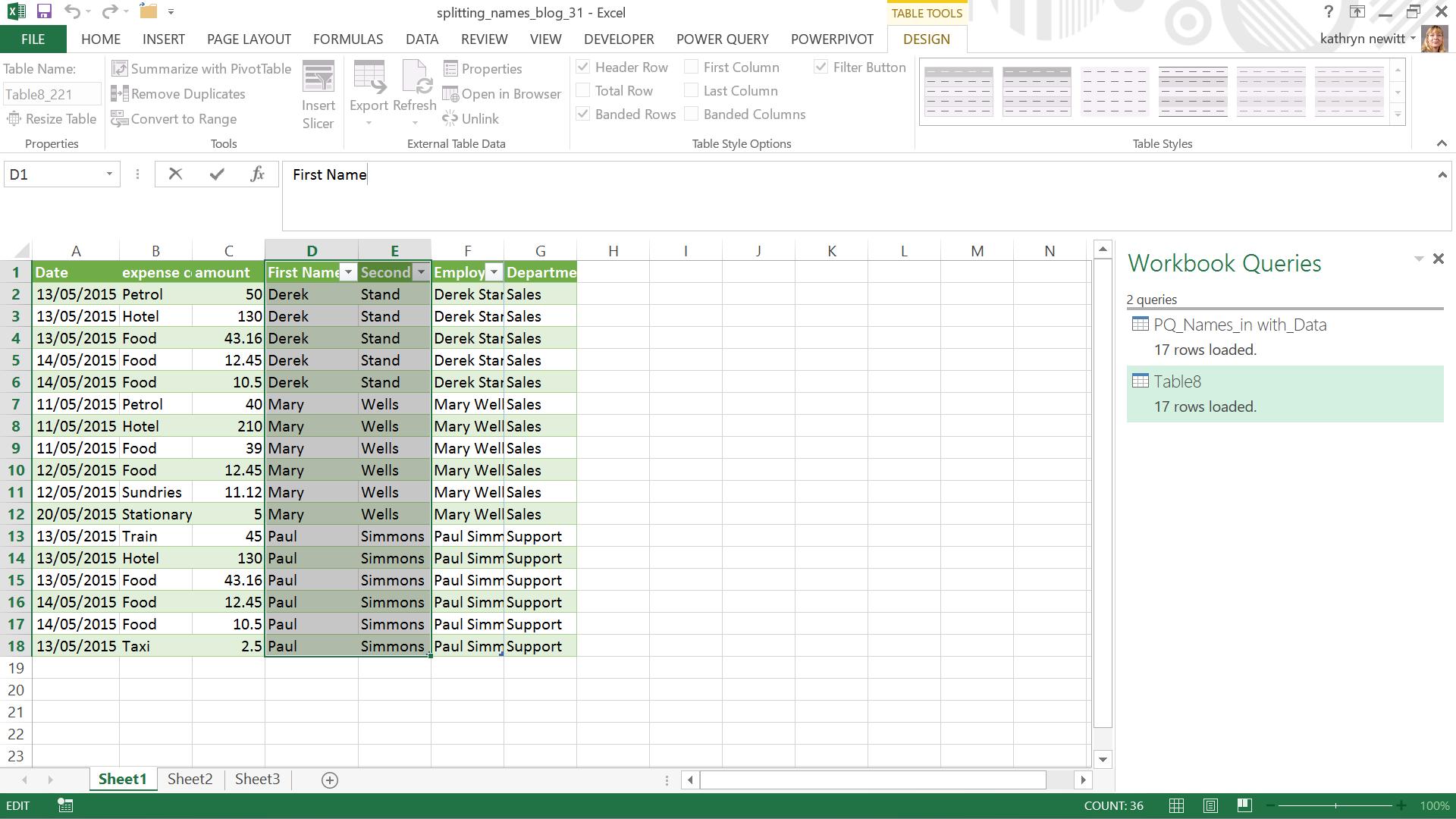
Since my data is already in a table, I take a copy and convert it to a range by using ‘Convert to Range’ option on the ‘TABLE TOOLS DESIGN’ tab (sorry for the shouting – I continue to use Excel 2013 for my examples!). Otherwise, Power Query will assume that the whole table should be loaded.
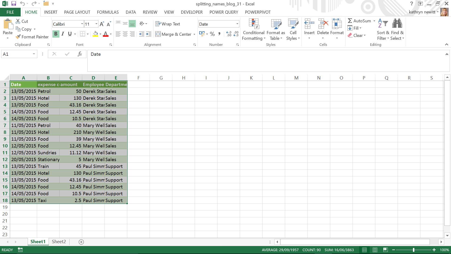
This gives me the range, which will no longer be connected to my ‘PQ_Names_in_with_Data’ query.
There are several approaches I could take. I could make my ‘Employees’ column an Excel table and load that, but I don’t actually need to take that step in Excel. Instead, on the ‘POWER QUERY’ tab, I choose the ‘From Excel Range/Table’ option. If I don’t specify my data by selecting it first, then Power Query prompts me to confirm the data I want to use:
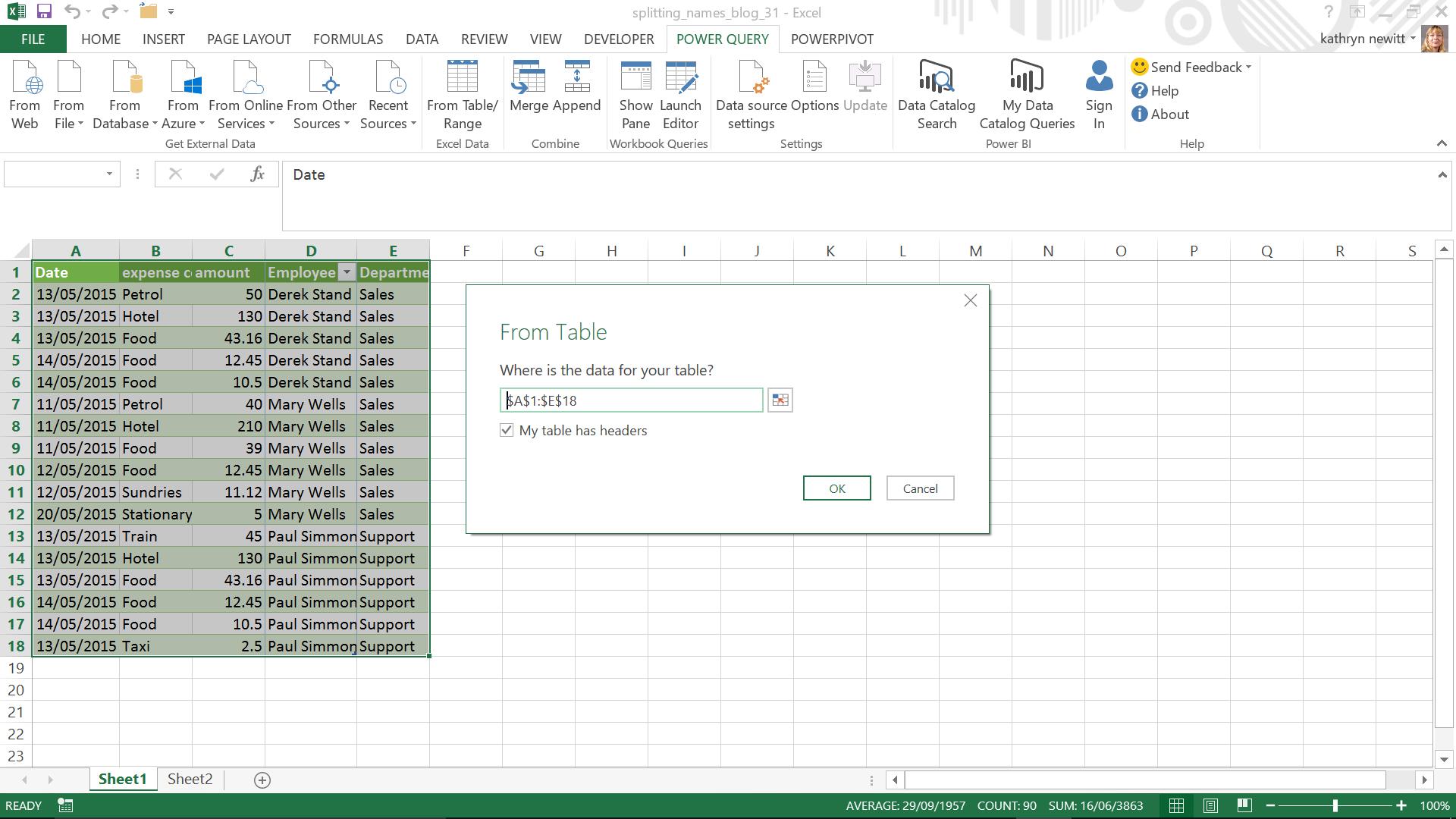
So I can either specify cells D1:D18 on here or I can select those cells first and Power Query will automatically load them.
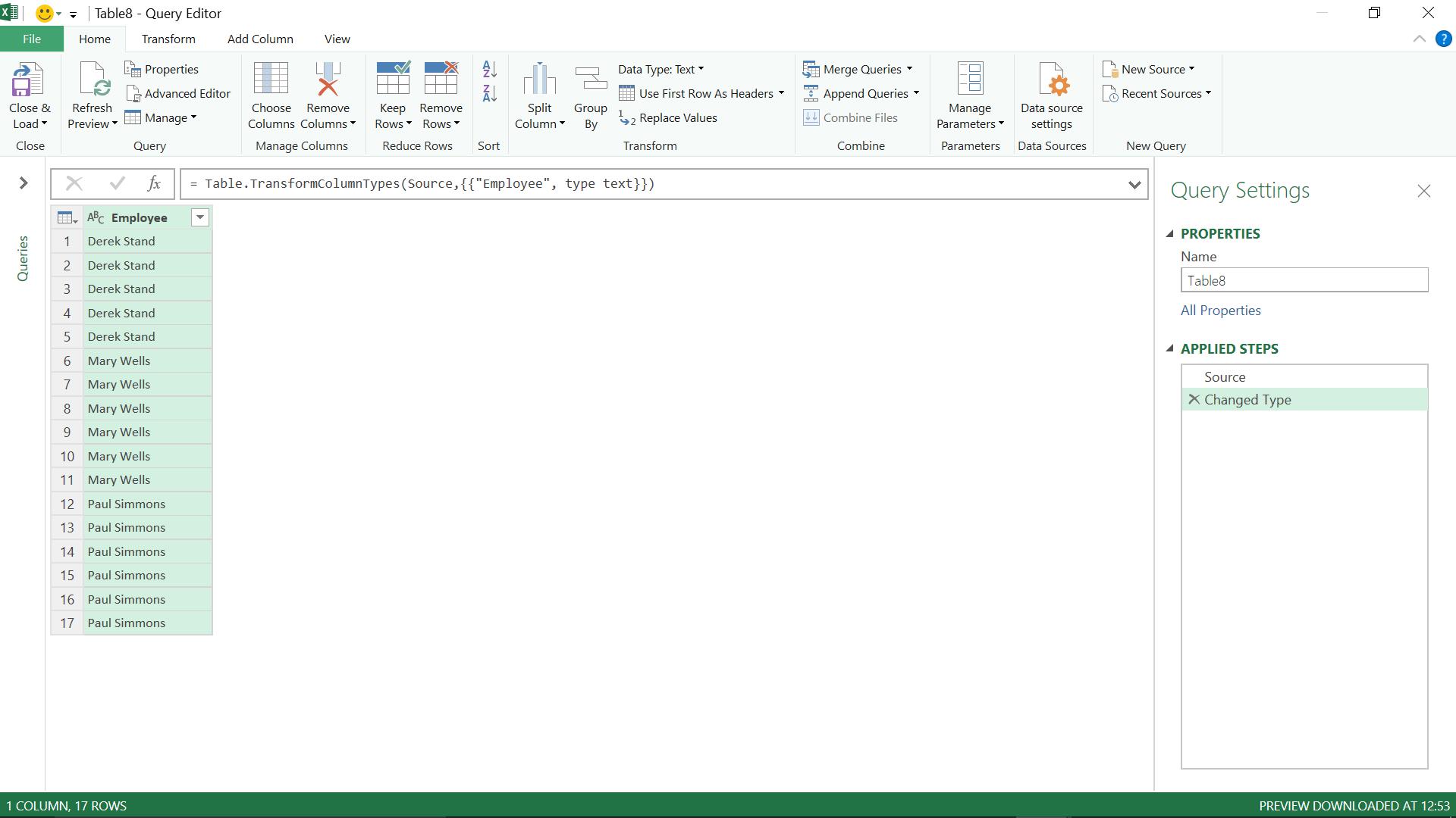
I now have my little table of data, and I am ready to split up the name.
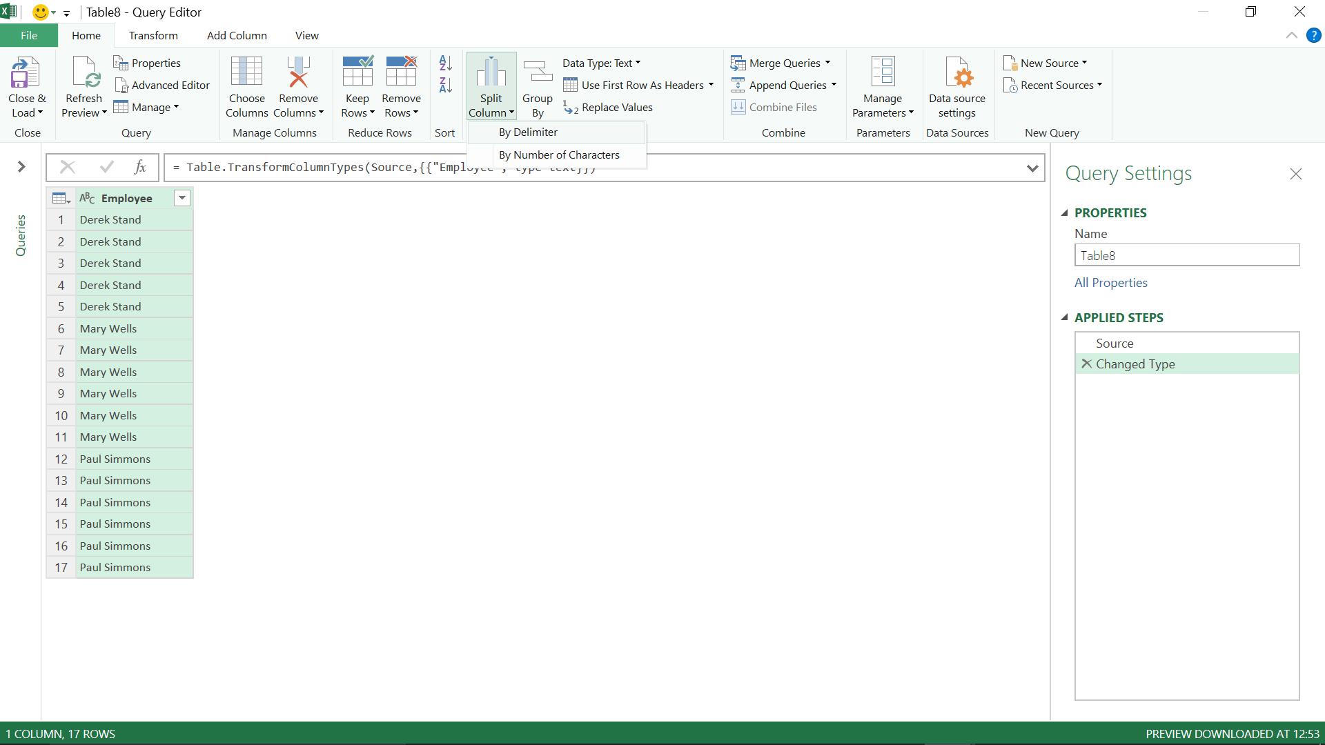
On the ‘Home’ tab, there is an option to ‘Split Column’, and I can choose to do this ‘By Delimiter’ or ‘By Number of Characters’.
I choose to split by delimiter, and the ‘Split Column by Delimiter’ screen appears. Power Query has correctly assumed ‘Space’ is my delimiter, but it’s worth taking a look at the other options:
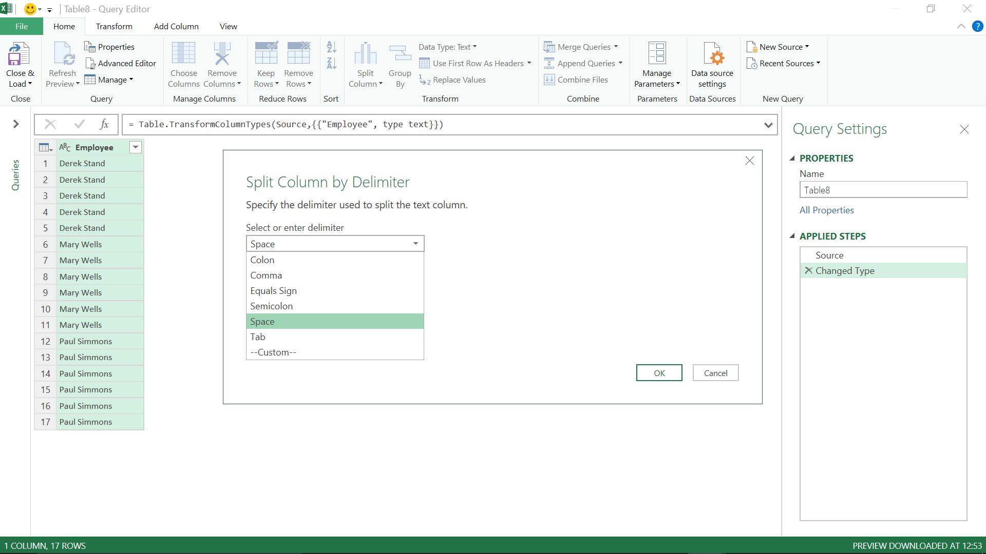
The most common options are explicitly listed and there is an option to customise my own delimiter for more complex data arrangements.
Also on the screen are a couple of other options:
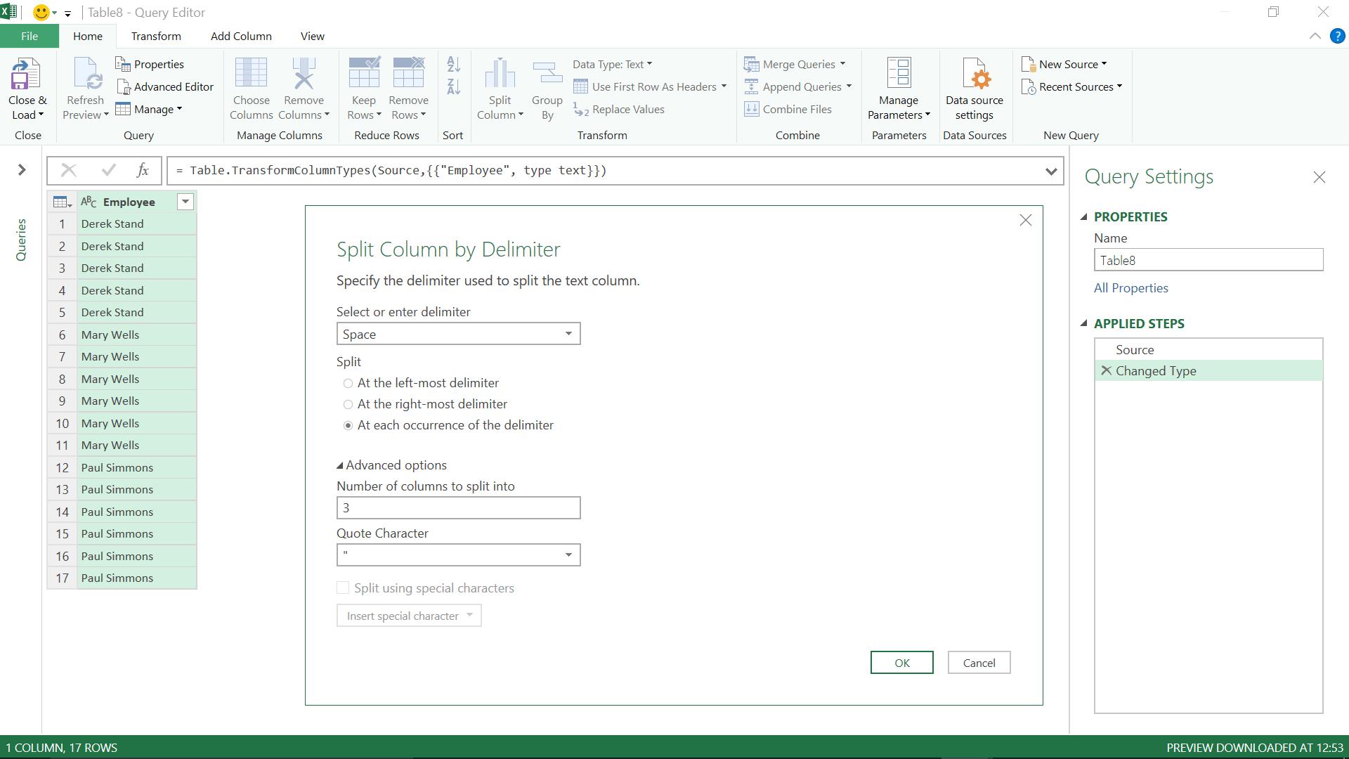
I can choose how often to split my data using the delimiter – this would be useful if some of the names included a first and second name as well as a surname, in which case I could choose to keep the first two names together by only splitting at the right-most delimiter. There are also some advanced options which allow me to specify how many columns I want to see. If I were to choose one then I’d only see the first name, if I choose three, the last one would contain null data. I can also choose the quote style. If I had special characters in my columns I could also choose to use them as a delimiter.
I am happy that I want to use the space as my delimiter and I will split each time I see a space (since I know that my data only has one space anyway). I choose to output to two columns.
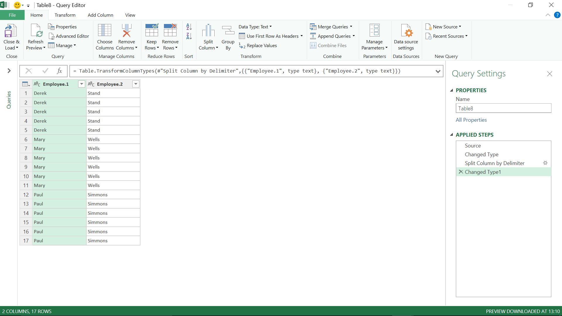
My two new columns are named ‘Employee.1’ and ‘Employee.2’, and I opt to ‘Close and Load’ which will load them to a new worksheet in my book. I rename them and insert my new columns into my original worksheet. Easy!
Want to read more about Power Query? A complete list of all our Power Query blogs can be found here. Come back next time for more ways to use Power Query!