Power Query: See it, Save it, Sort it - Part 1

Welcome to our Power Query blog.  This week, I begin looking at a sorting issue, by initially considering Best Practice when extracting my data.

I have some data for my imaginary salespeople (I know you were missing them!).

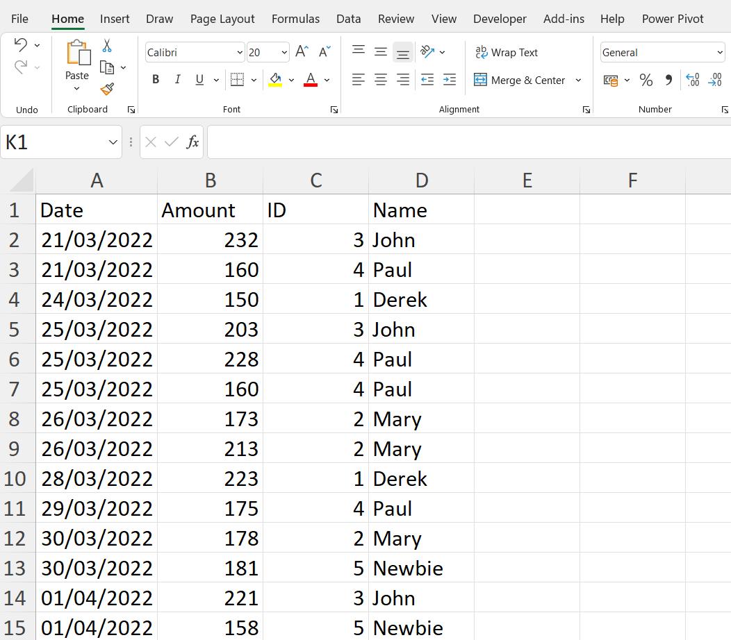
I am going to be performing some calculations with my data, but first I need to transform it. When I transform the data, Power Query will convert the data I select into a Table.  Tables have columns of consitent data, e.g. the Date column contains dates, which means that formulae or calculations apply to every value in a column.  

I am going to create the Table myself by selecting all my data and using CTRL + T (I could also achieve this by using ‘Insert Table’ from the Insert tab).  I want to create a Table first so that I can name the Table before it is extracted.  This is Best Practice because it makes it easier to determine the link between queries and Tables, and makes my model more consistent.

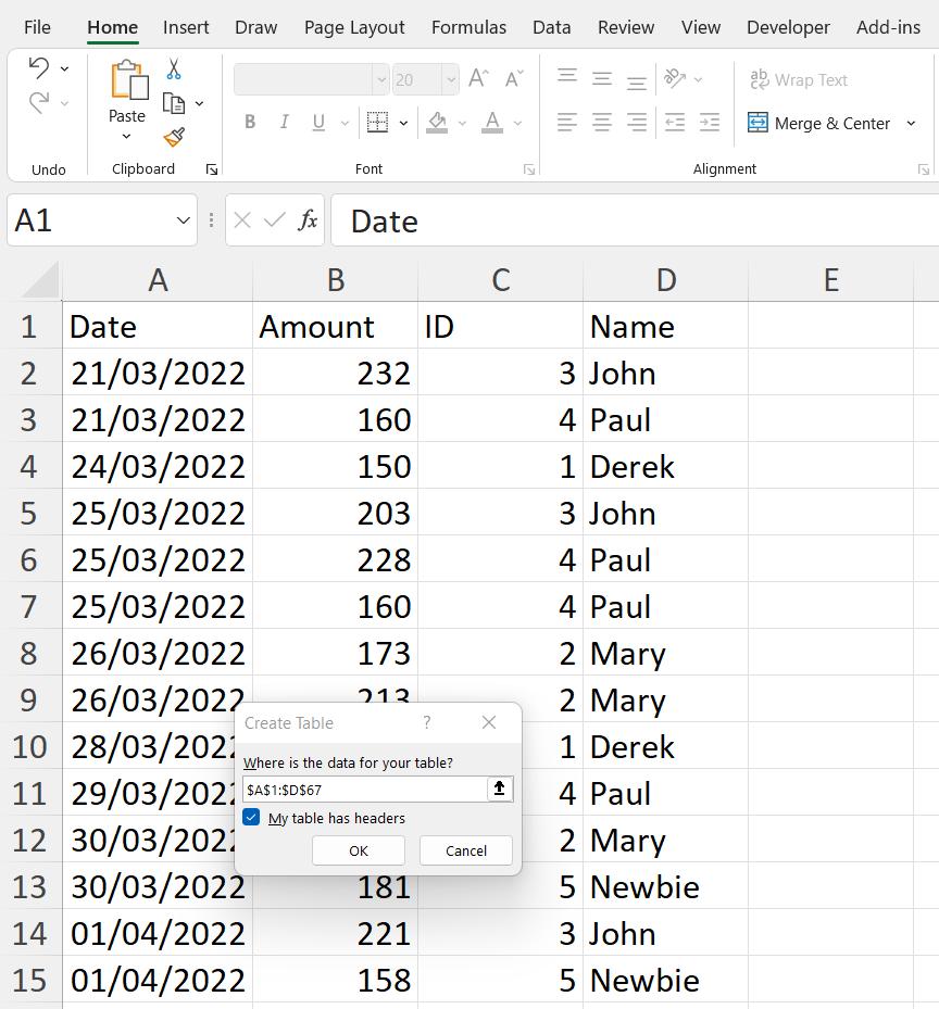
Excel has decided that ‘My table has headers’.  Headers are detected by comparing the first row in the data with the rows underneath.  If the Data Types in the first row differ from the other rows, then Excel assumes I have headers.  Since I have dates and numbers in my selected data, Excel has correctly determined that since the first row contains text values, hence I must have headings.

I click OK, and the Table is created.  The Table tab is now available on the Ribbon when I am in the Table:

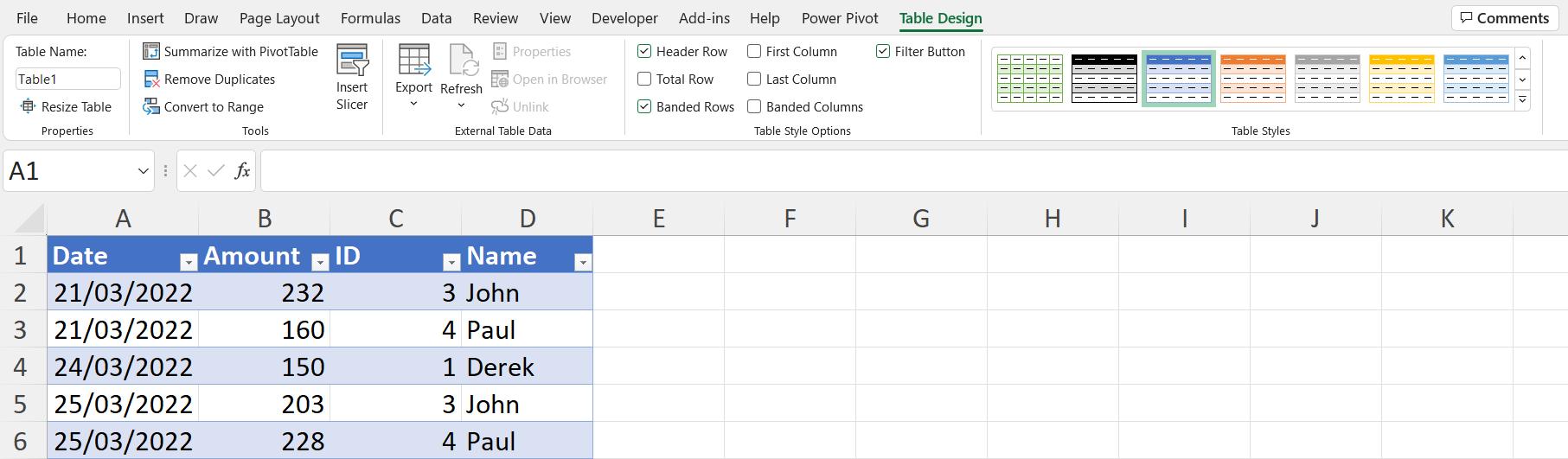
On the top left is a ‘Table Name’ title, and underneath that I can see my Table is currently called ‘Table1’.  I can change this to something more meaningful: I call it Sales_Transactions (the final ‘s’ is beyond the size of the ‘Table Name’ window).  

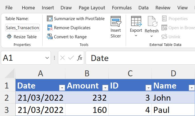
Note that an Excel Table name can’t have spaces in it, which is why I have used the underscore (_).  Now I click anywhere in the Sales_Transactions Table, and use ‘From Table/Range’ in the ‘Get & Transform’ section of the Data tab:  

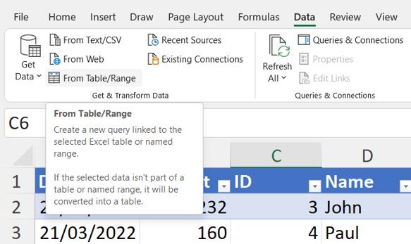
Since my data is already in a Table, this takes me directly to the Power Query editor:  

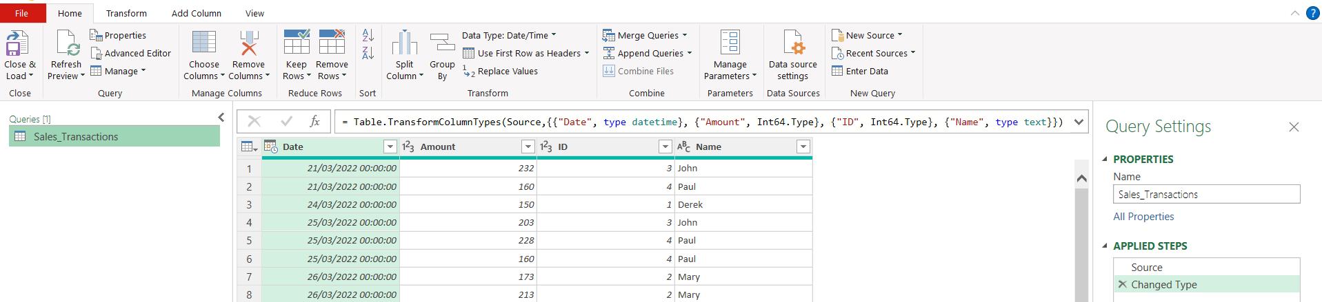
My Power Query table has the same name as the Excel Table, which makes it easier to trace where the data is coming from.  If I hadn’t done this, I would have to use the Source step to locate my data:  

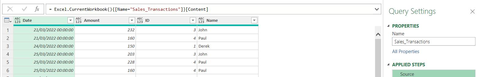
The M code for this step is:  

where [Name="Sales_Transactions"] Identifies the name of the Excel Table.

Now I have my data in Power Query, I want to ensure that I have a row for every date, as I plan to apply time intelligence calculations to my data.  To do this, I am going to create a list of all dates that I can append to my data.  More on this next time!

Come back next time for more ways to use Power Query!