Power Query: Picky Pivoting

Welcome to our Power Query blog. This week, I look at unpivoting data with multiple headings.

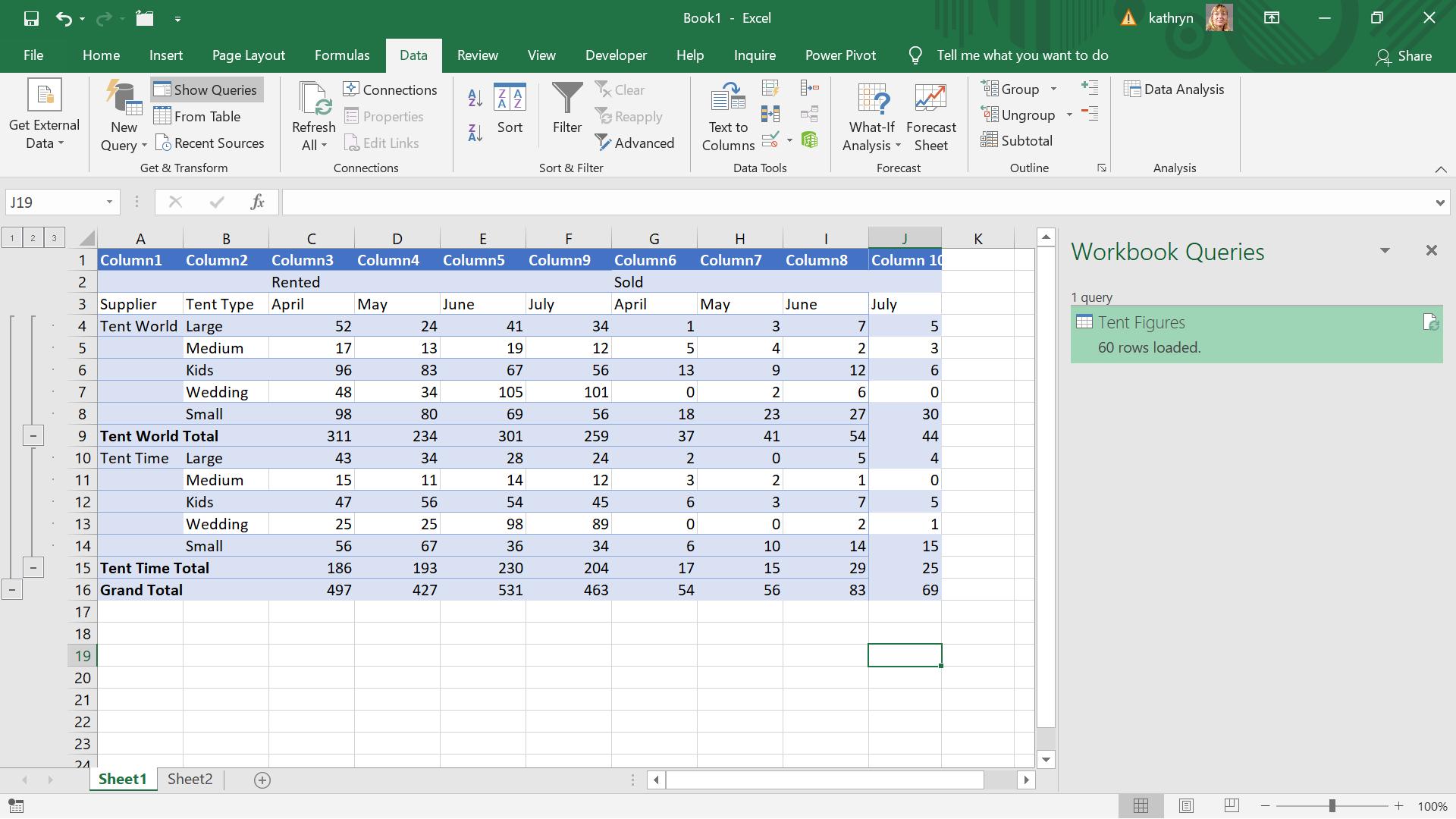
I have some tent data:

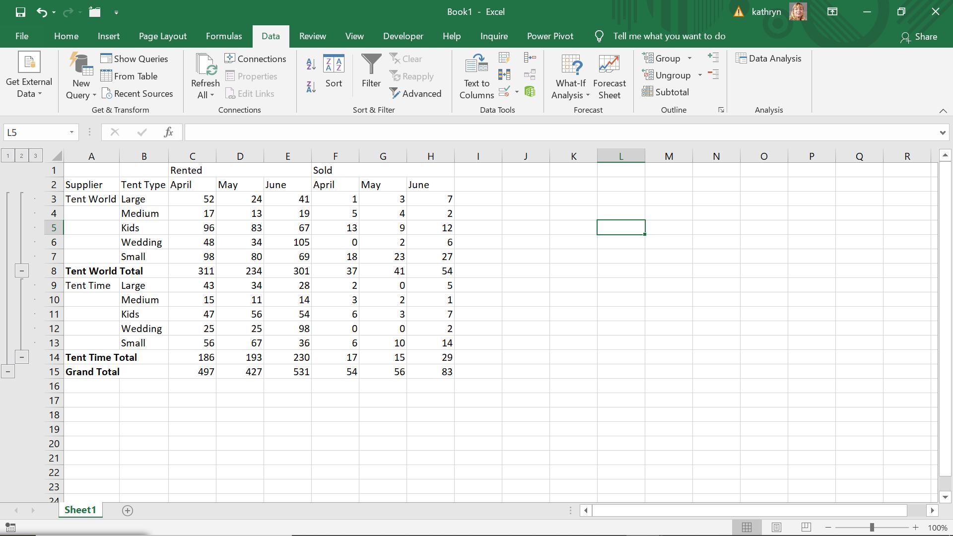
I want to get this data into a standard table format so that I can analyse it and combine it with other data. I want to do this in a dynamic way, so that if more months are added to my Excel sheet, then the data will be transformed correctly.

I start by extracting the data to Power Query by selecting ‘From Table’ in the ‘Get & Transform’ section of the Data tab.

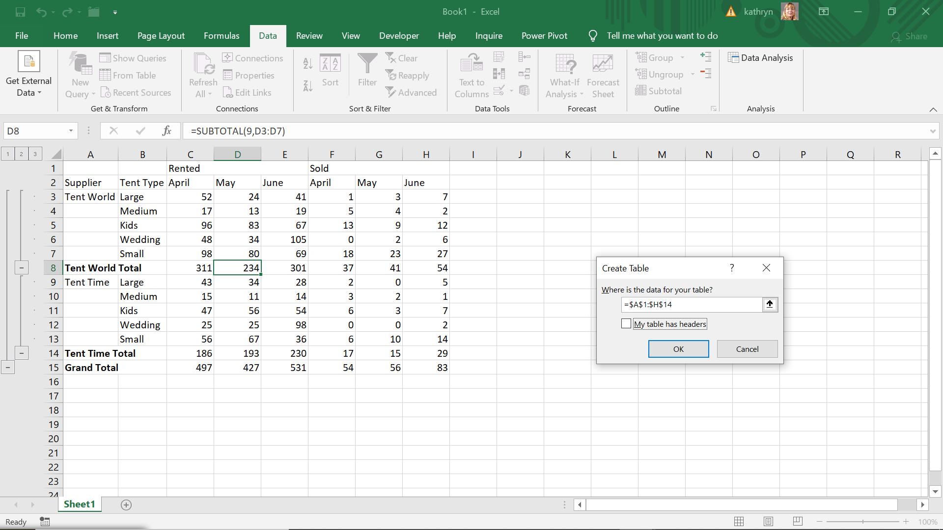
Power Query automatically selects my data without the ‘Grand Total’ line, and this is fine for my purposes. I choose not to select the ‘My table has headers’ box as it wouldn’t find the correct headers in any case.

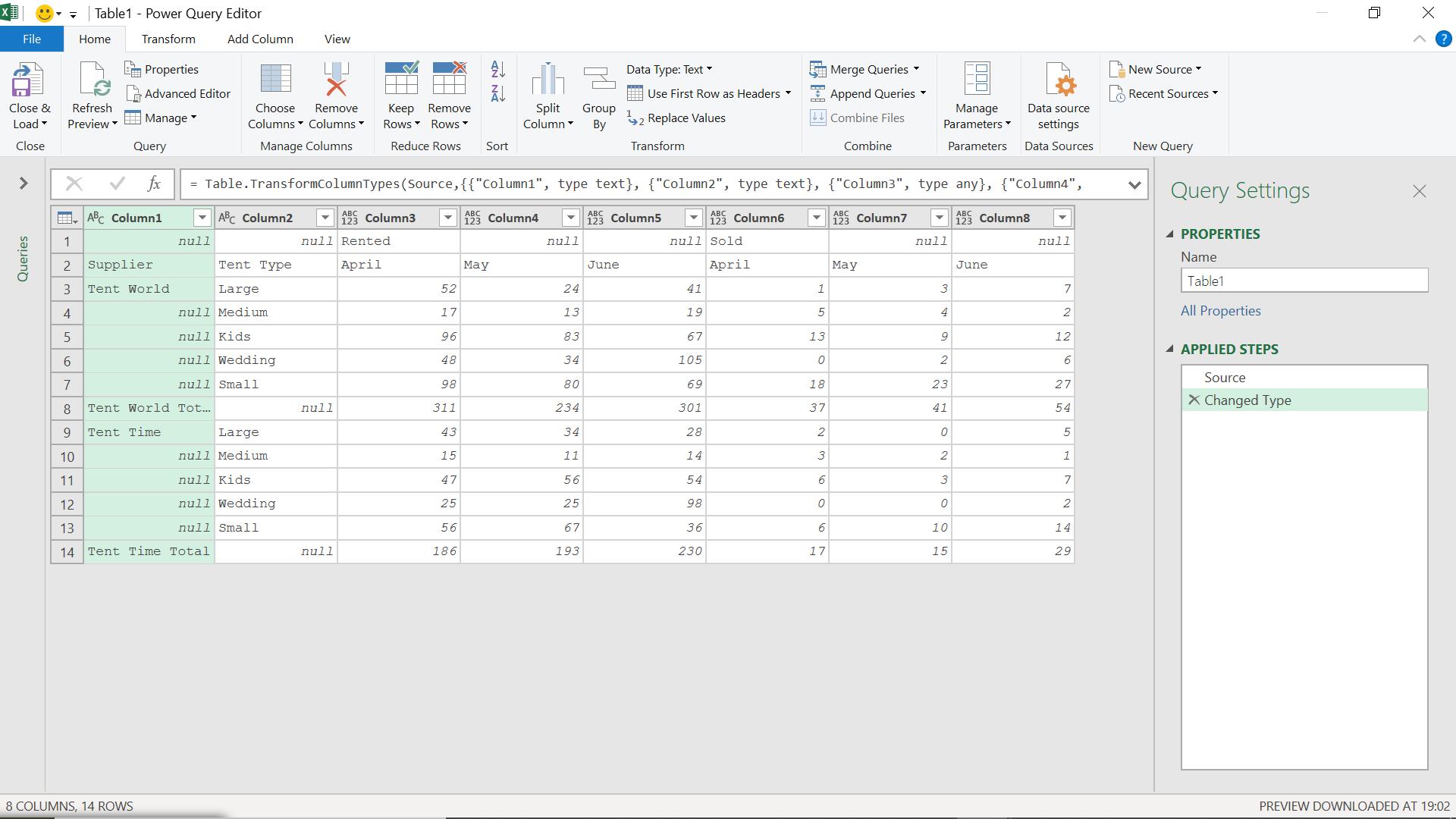
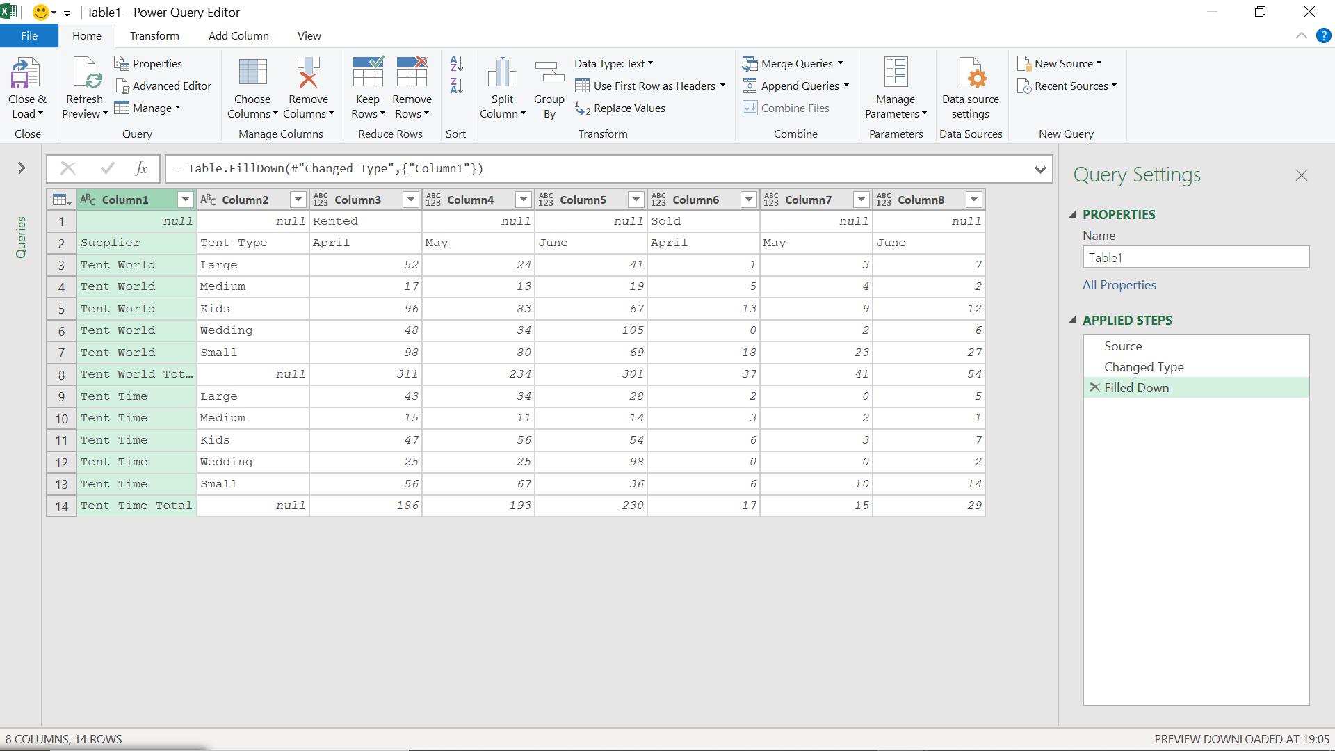
I start by sorting out my supplier data, so I right click on Column1 and choose to ‘Fill Down’.

I know that I want to keep the supplier data and the tent type data, so I choose to combine these columns. The remaining columns will need more manipulation to sort out the headings.

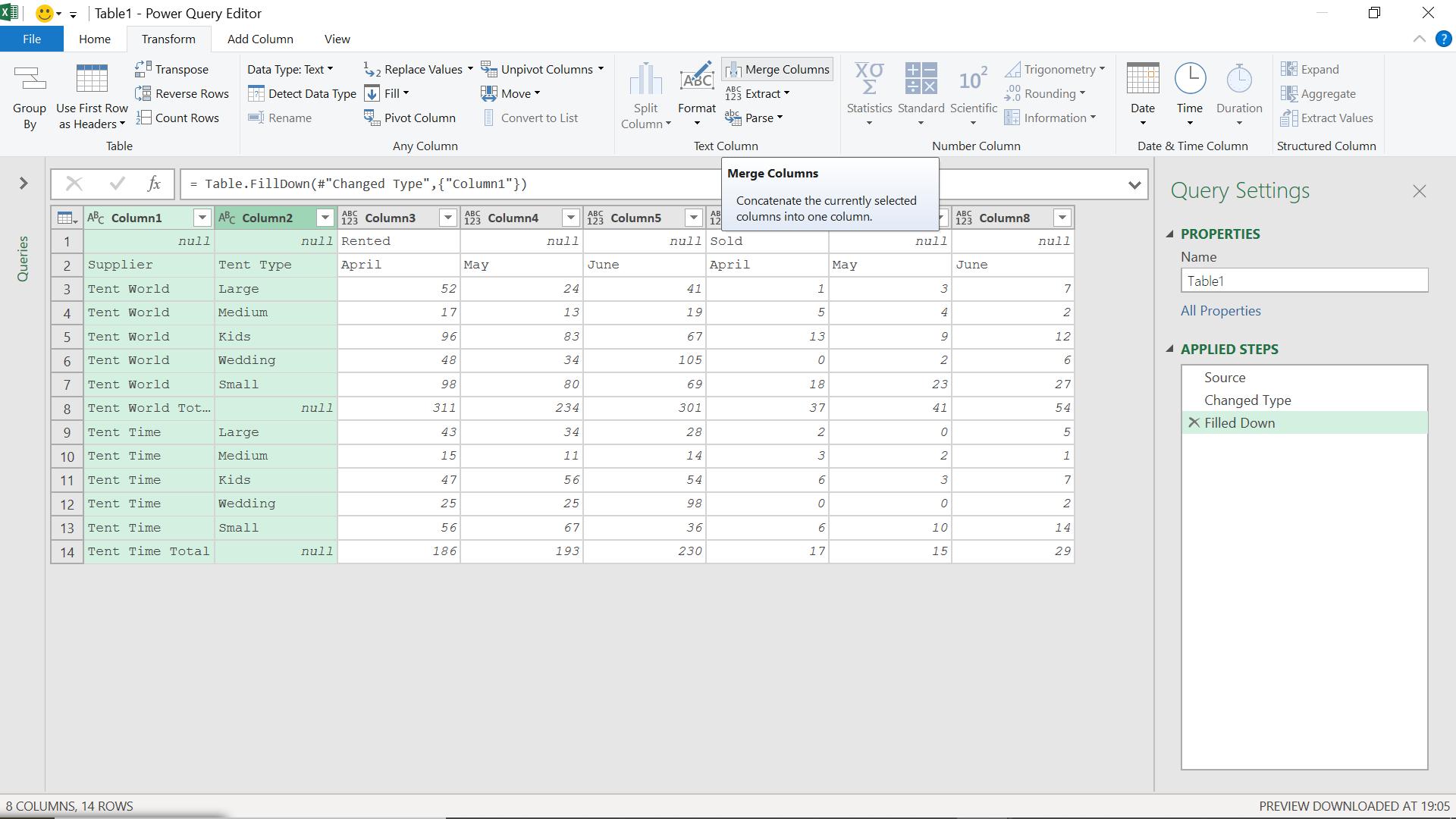
On the Transform tab, I can select Column1 and Column2 and choose to ‘Merge Columns’.

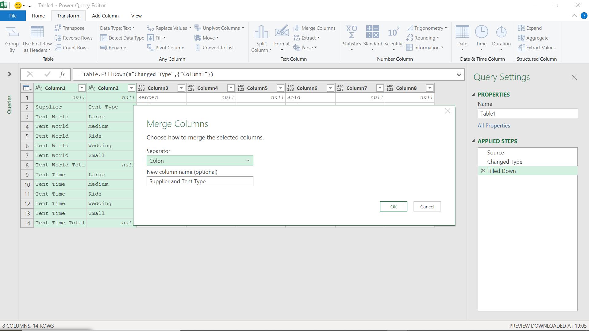
I choose to separate my data by a colon (:), and use a meaningful name for my column name.

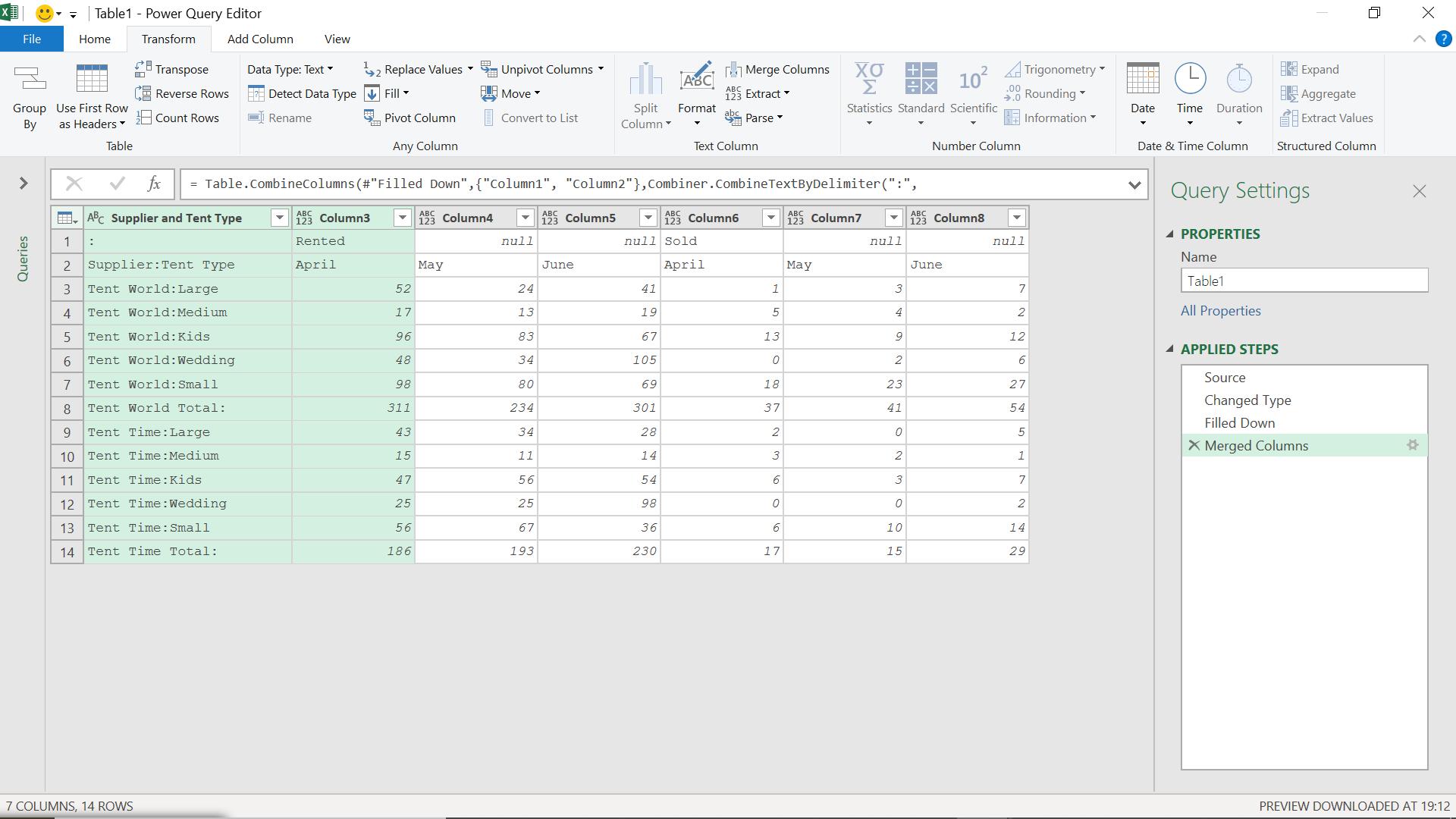
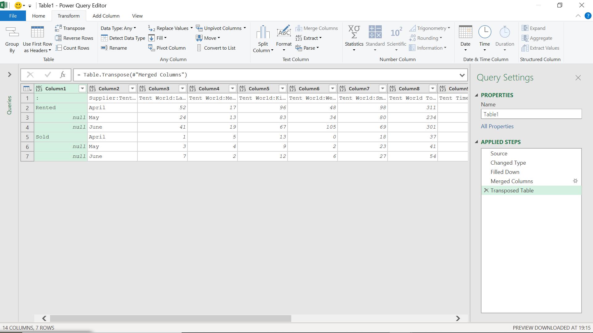
On the Transform tab, I also have the option to ‘Transpose’ my data, which will treat columns as rows and rows as columns.

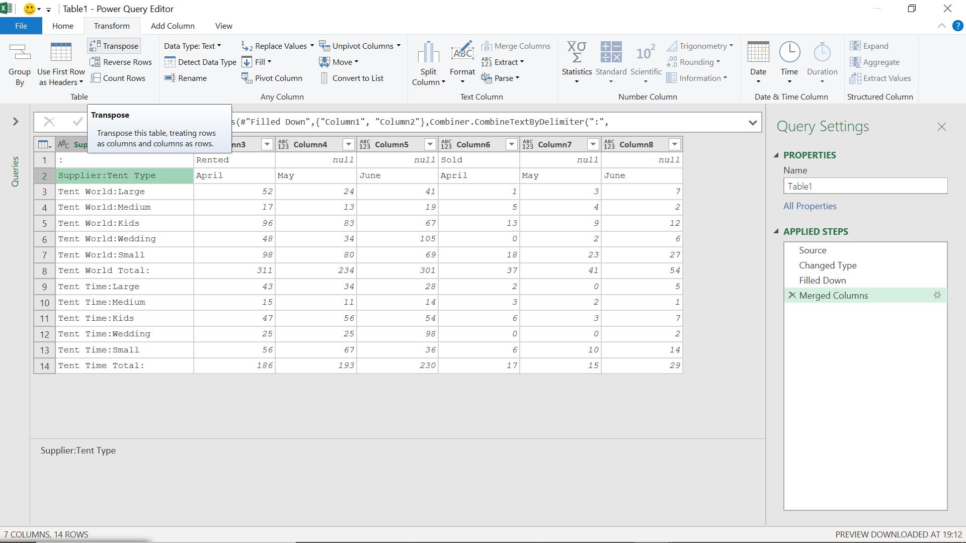
When I click ‘Transpose’, my data is swapped around:

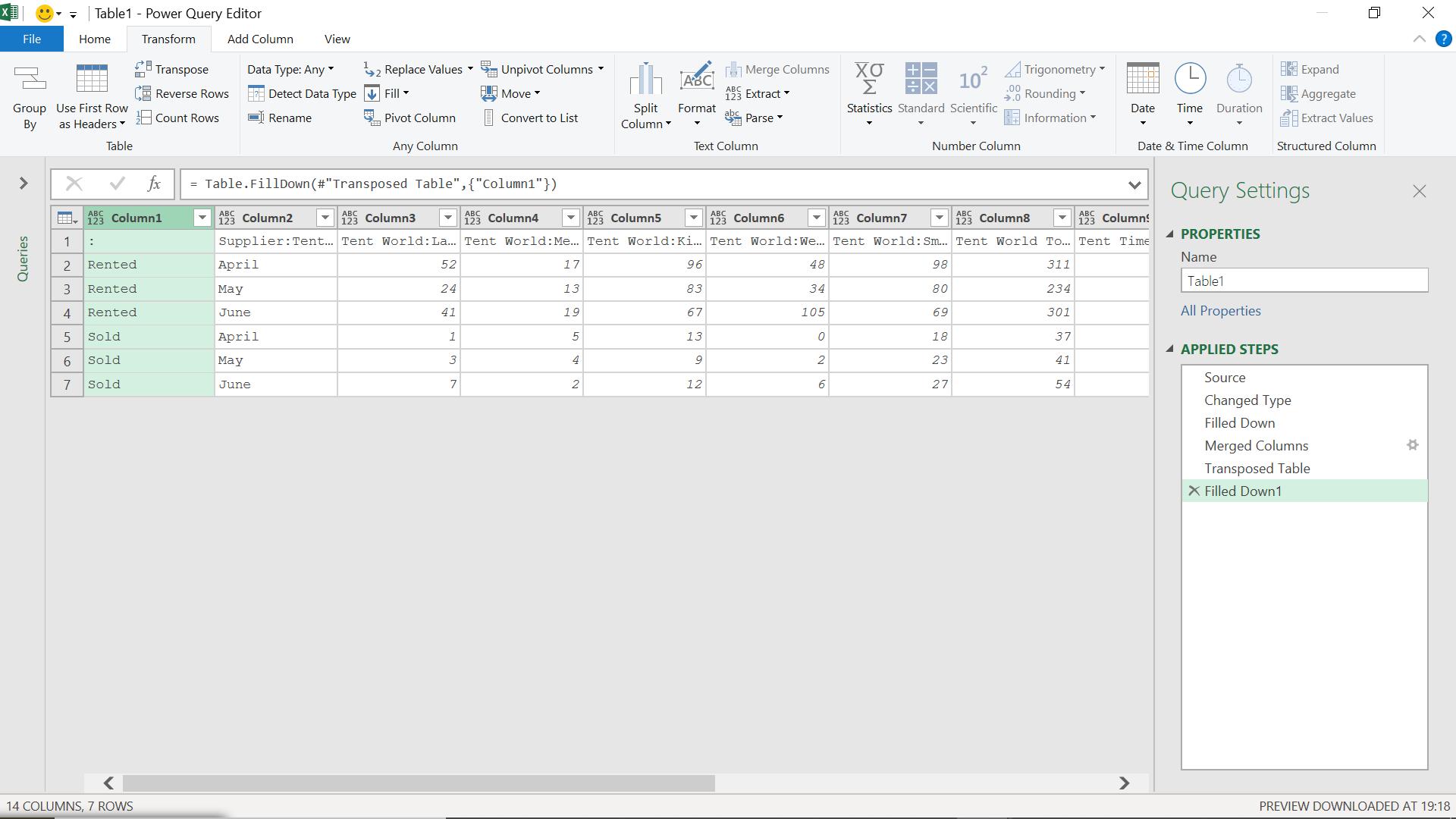
Next, I need to fill down the data in my first column so that ‘Rented’ or ‘Sold’ appears next to each month.

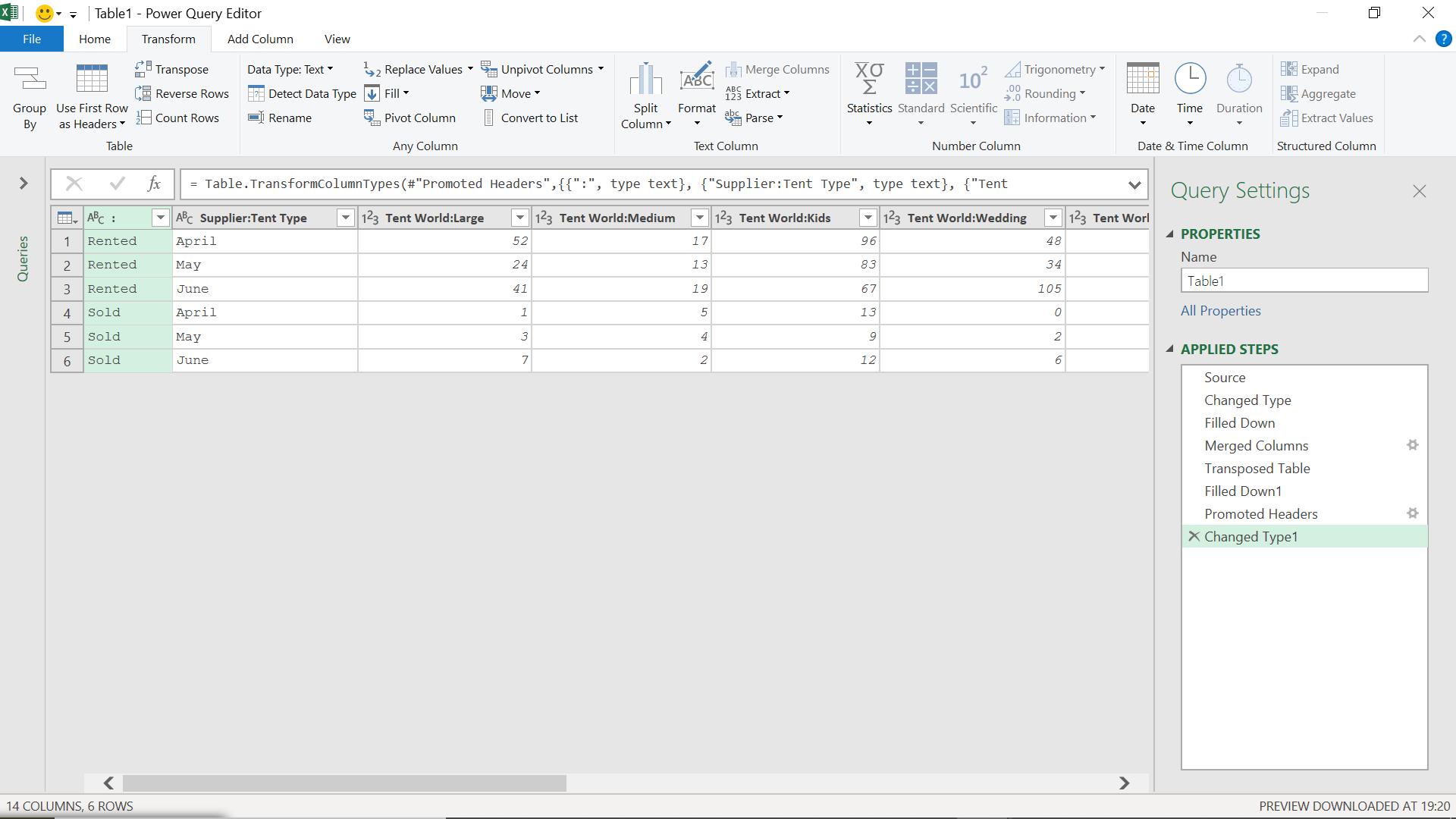
Now, I can promote the row with the supplier and tent type information to be my headers from the ‘Use First Row as Headers’ section.

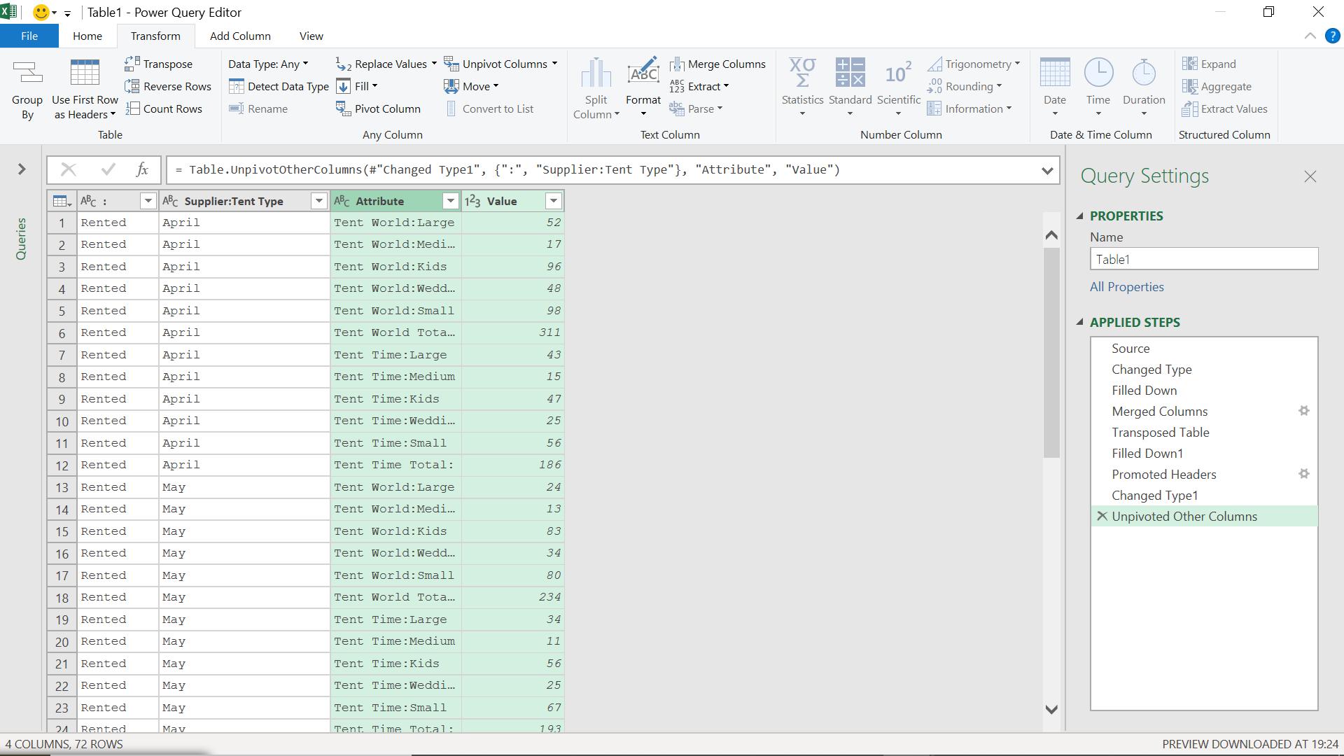
The data is already looking much better. I am ready to unpivot the quantities. I select the first column (Rented / Sold), and the Supplier:Tent Type column and choose to unpivot the other columns. I can do this by right clicking with my columns selected.

I can now split the Attribute column into my original columns.

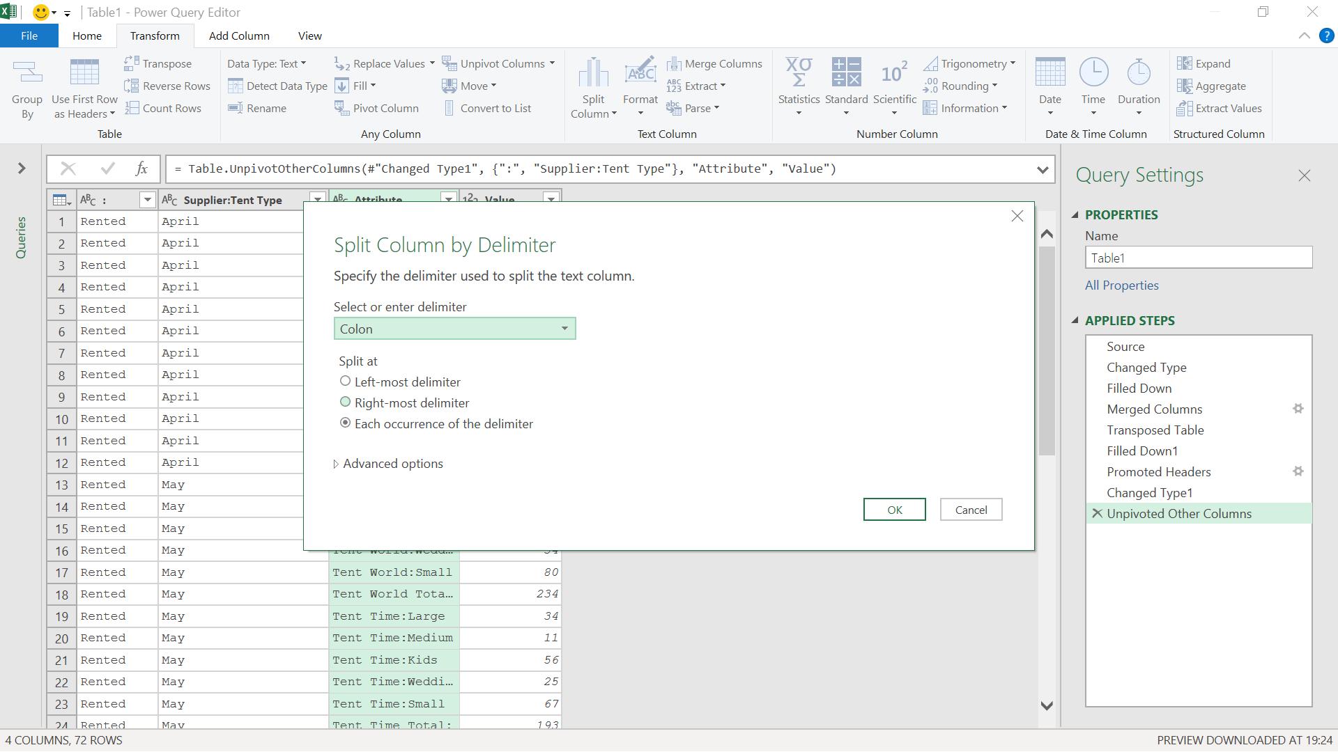
I choose to split by colon.

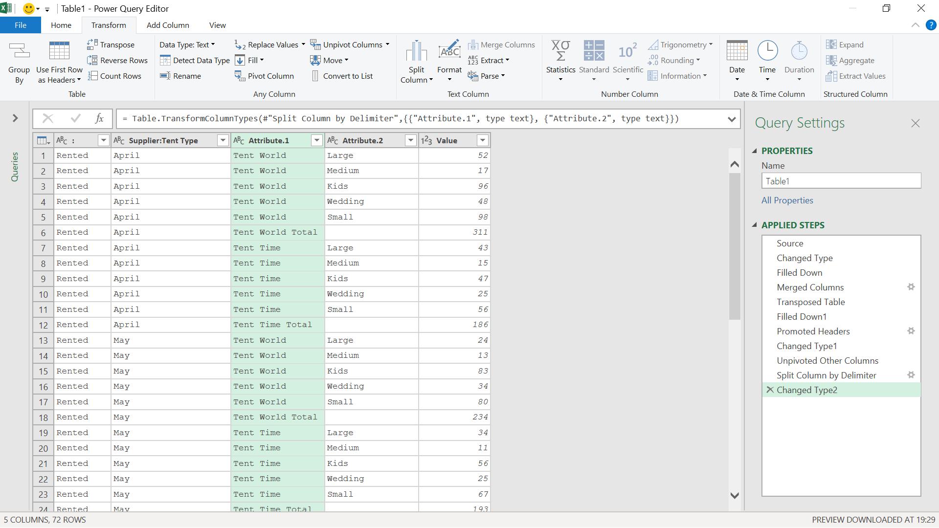
I can now rename my columns.

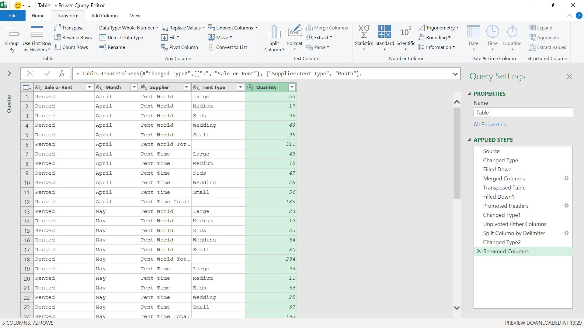
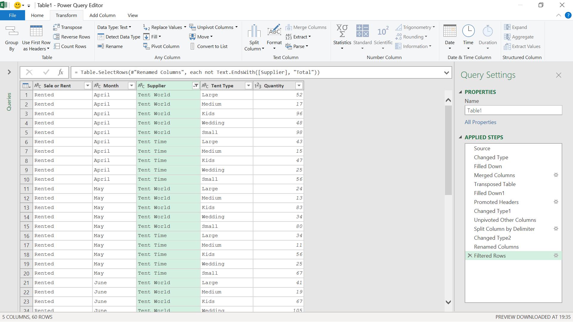
I remove my total rows by filtering on Supplier, looking for the word ‘Total’.

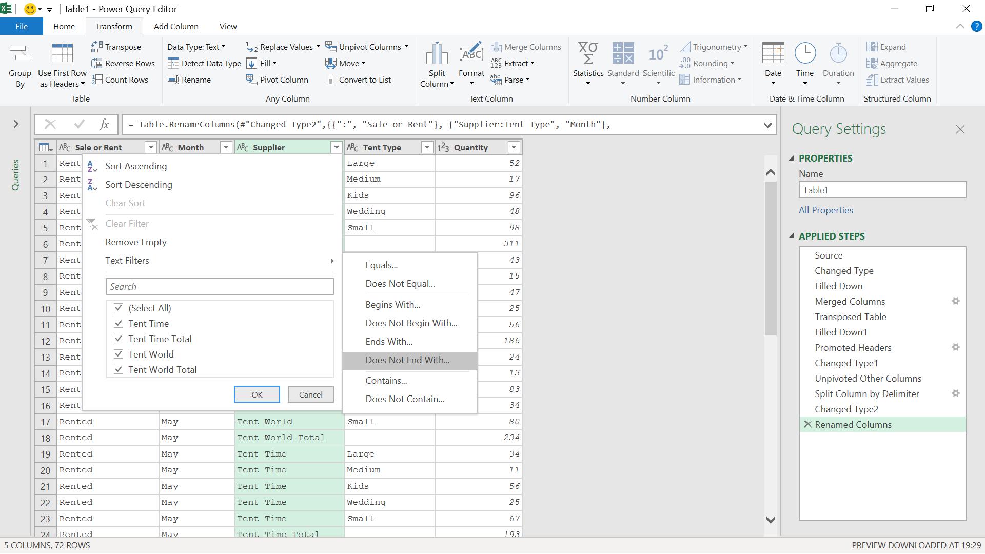
I choose ‘Does Not End With…’ just to reduce my chances of coinciding with an actual supplier name.

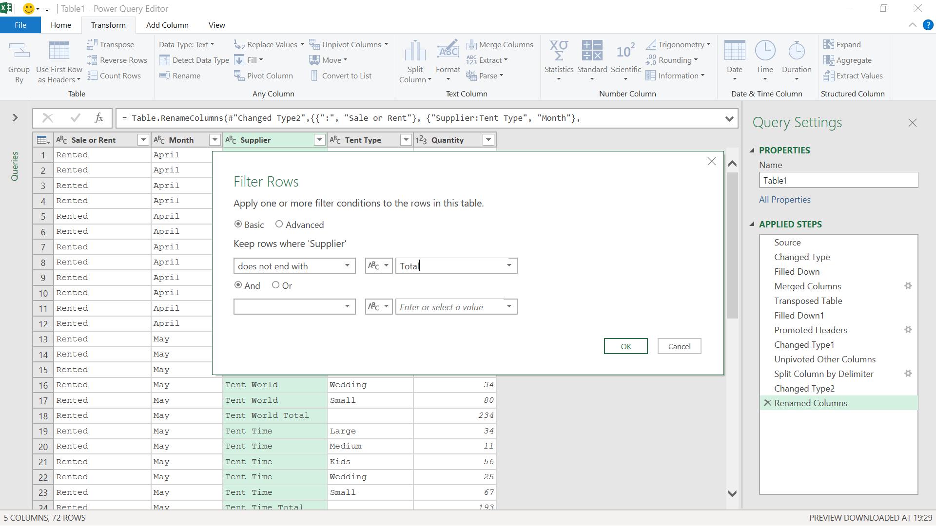
I click ‘OK’ to see my data.

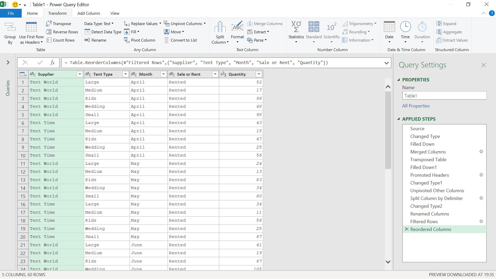
I reorder the columns.

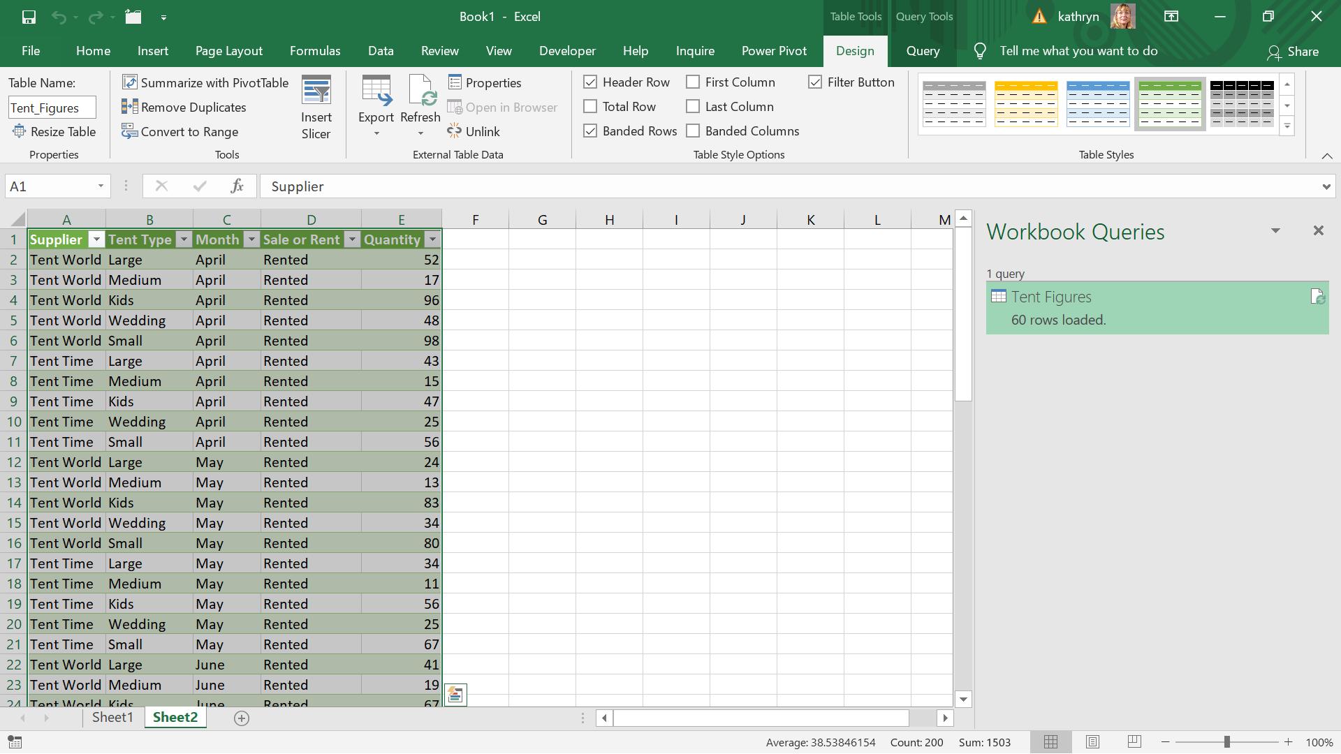
I can now use ‘Close & Load’ on the ‘Home’ tab to upload my data to Excel.

Finally, I need to add data for July to my original Excel spreadsheet to check my query still works.

I refresh my query and check the data.

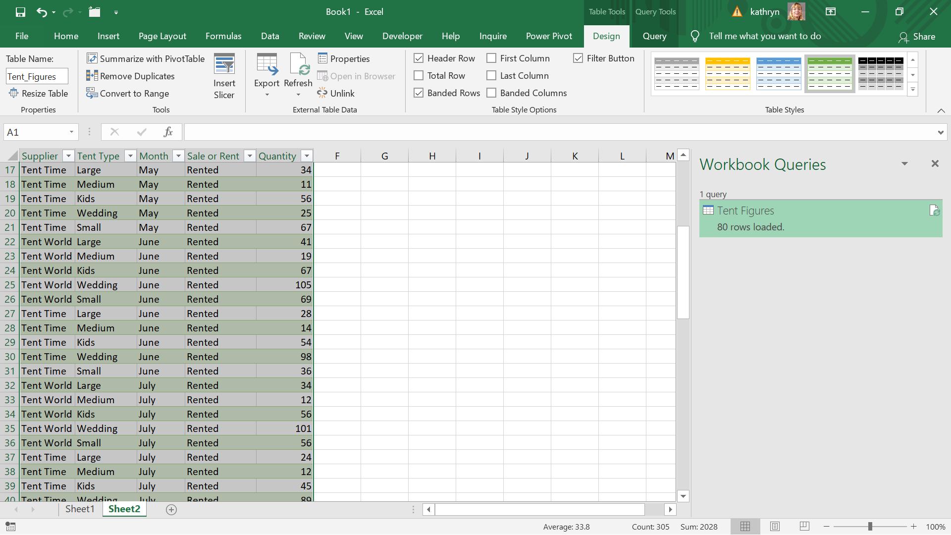
The data for July has been included.

Come back next time for more ways to use Power Query!