Power Query: Empty

Welcome to our Power Query blog. This week, I look at how to achieve the opposite of fill up / down.

Maureen is in charge of my imaginary salespeople. She has been looking at the following data and she has a request…

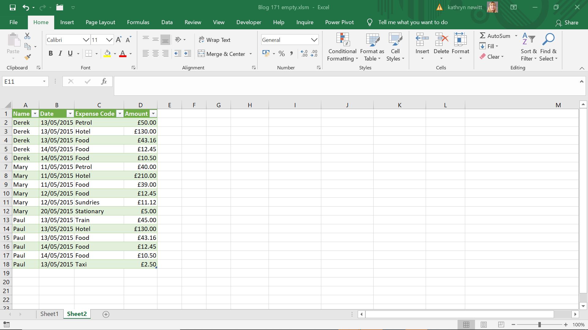
Maureen doesn’t want to see the salesperson’s name on each row, she wants to only see it on the first row for that salesperson. She’s not interested in PivotTables!

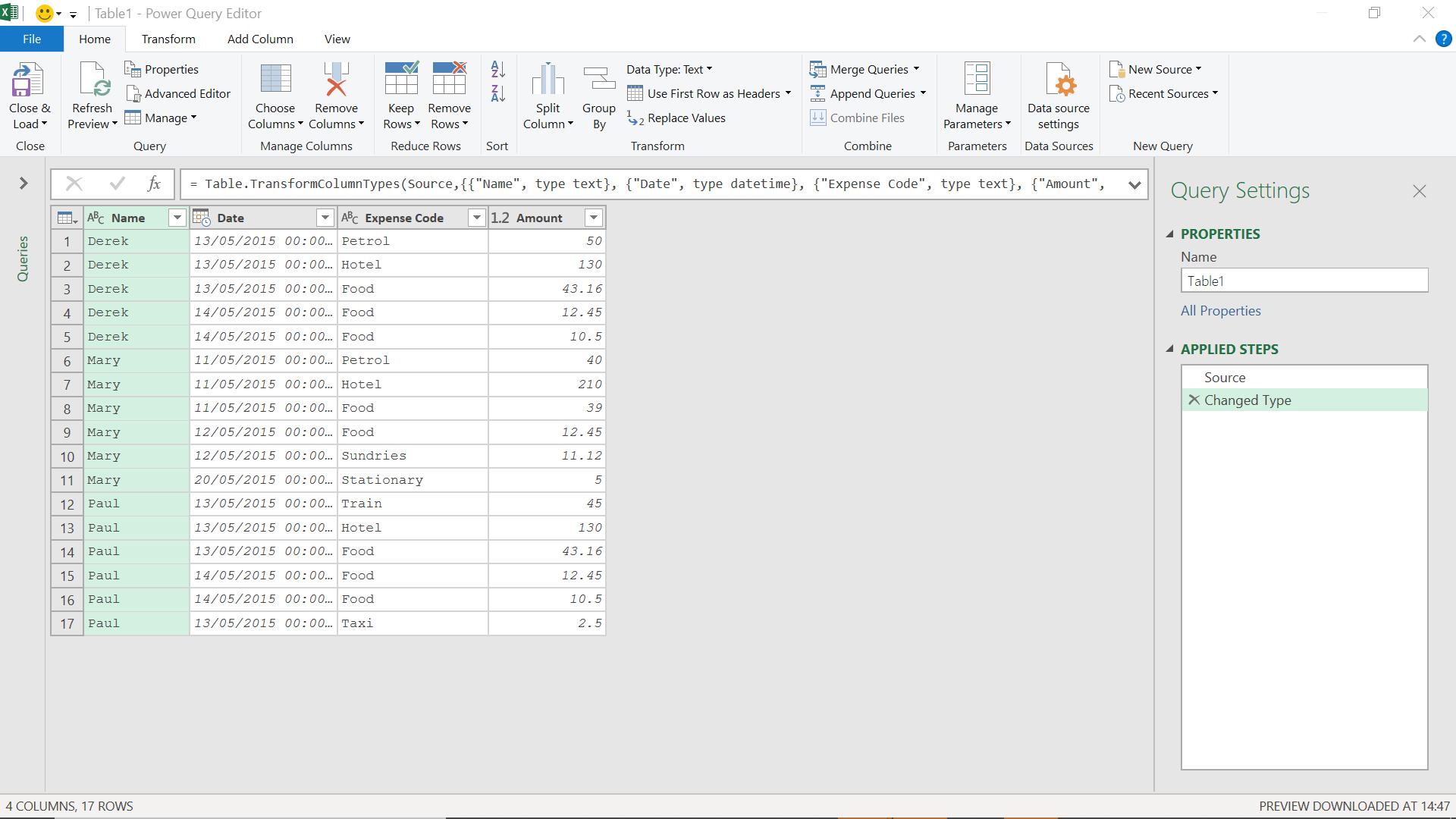
I begin by extracting the data to Power Query using the ‘From Table’ option on the ‘Get & Transform’ section of the Data tab.

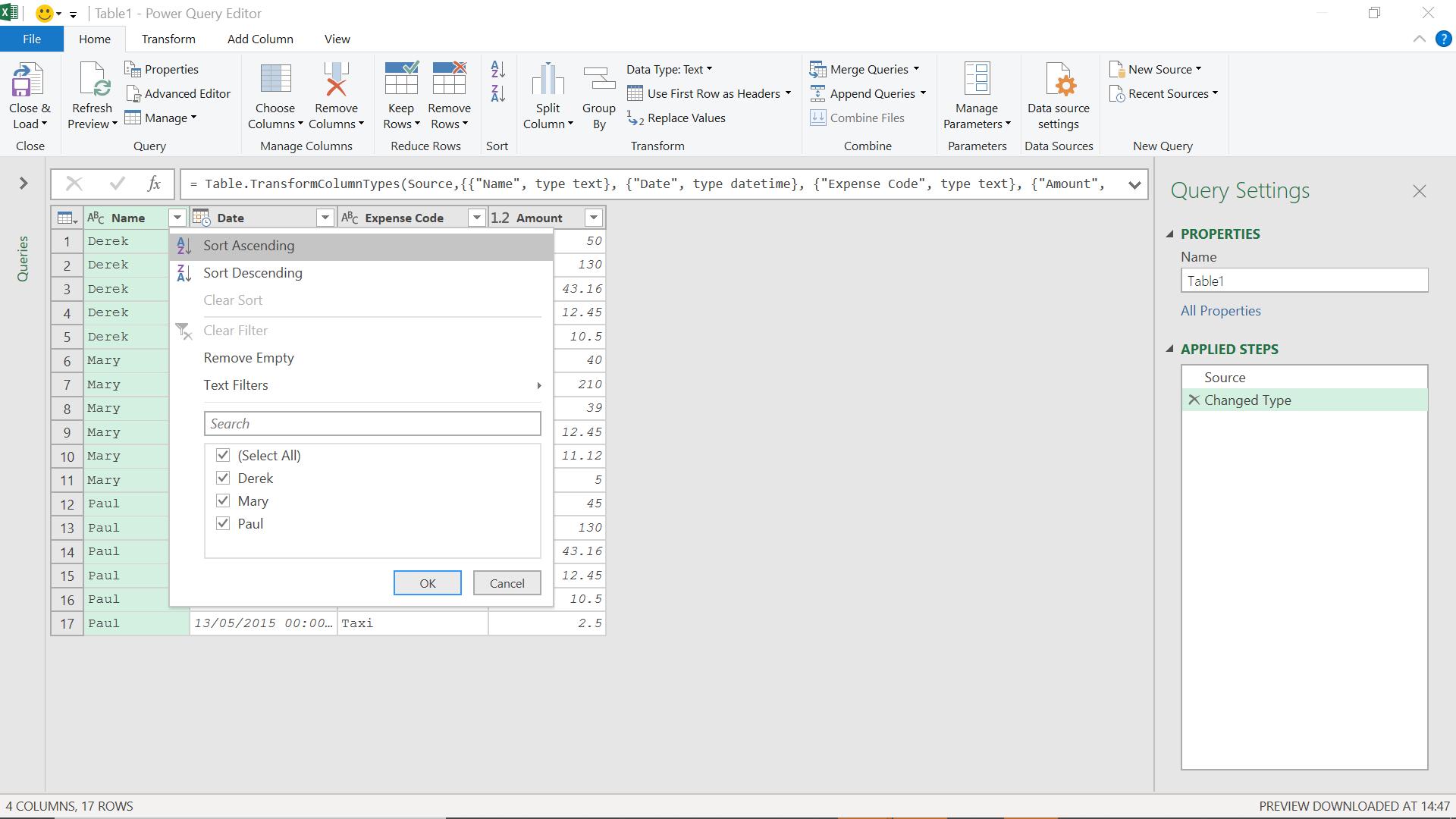
Since I want to essentially split my data into groups under each name, I start by sorting by name using the filter next to Name.

Having ordered by data, I need to group it. I can do this using ‘Group by’ on the Transform tab.

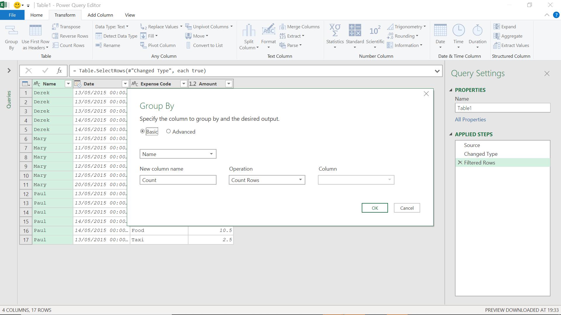
I include a simple aggregation to count all rows:

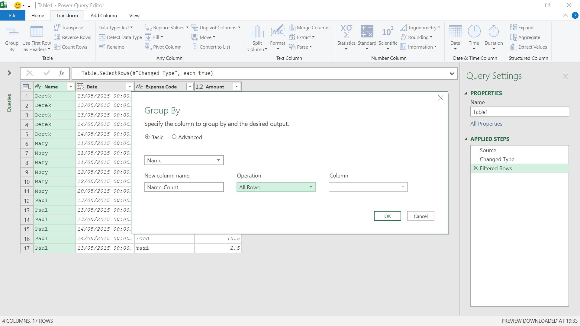
I click OK to see my grouping.

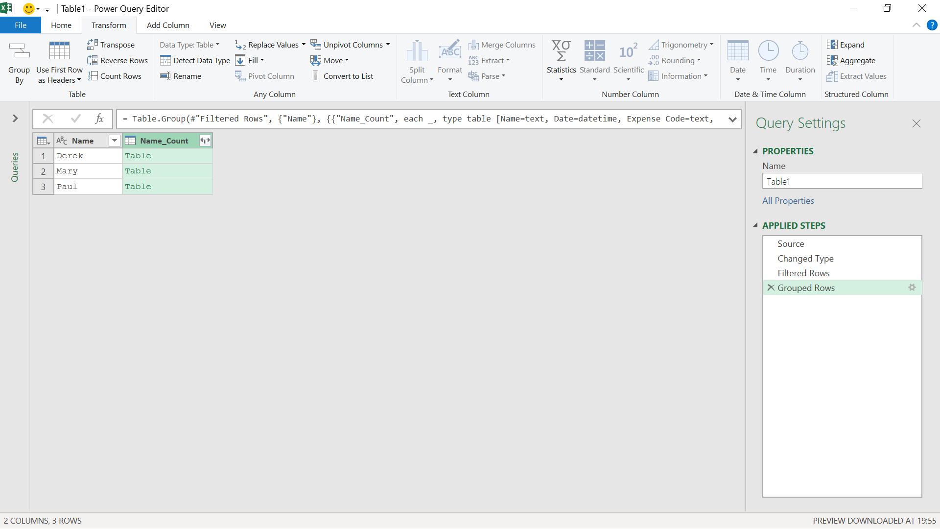
I now need a method of linking all the rows with the same name, so I use an index column. I want to effectively add an index column to each table in Name_Count so I do this by adding a ‘Custom Column’ from the ‘Add Column’ tab.

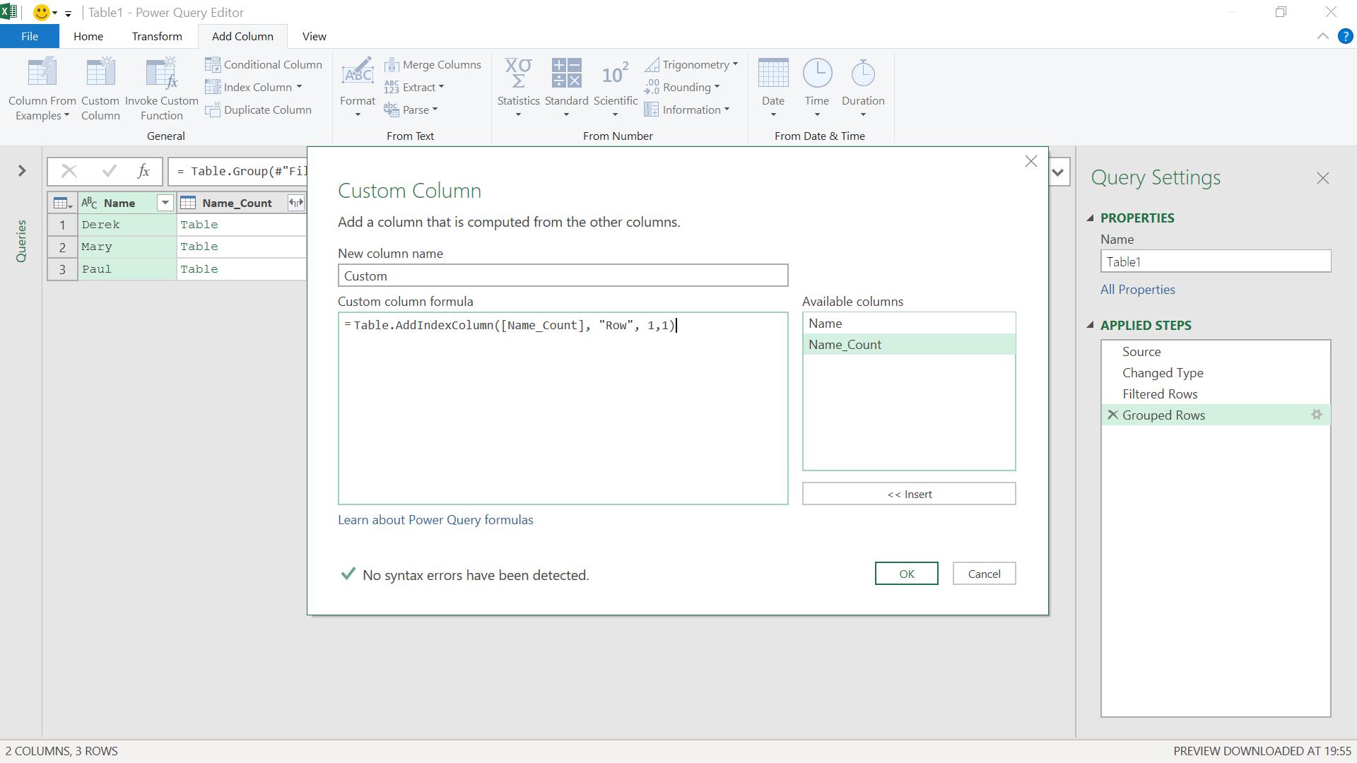
The M code I have used is:

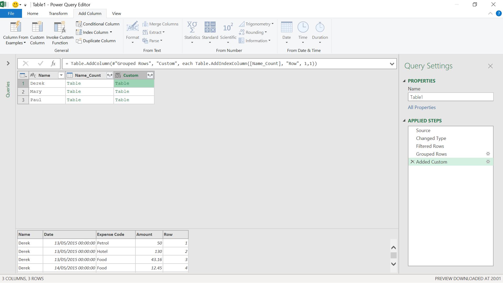
I can see that all my information is in my new Custom column, so I can remove the other columns by selecting Custom, right-clicking and choosing ‘Remove Other Columns’.

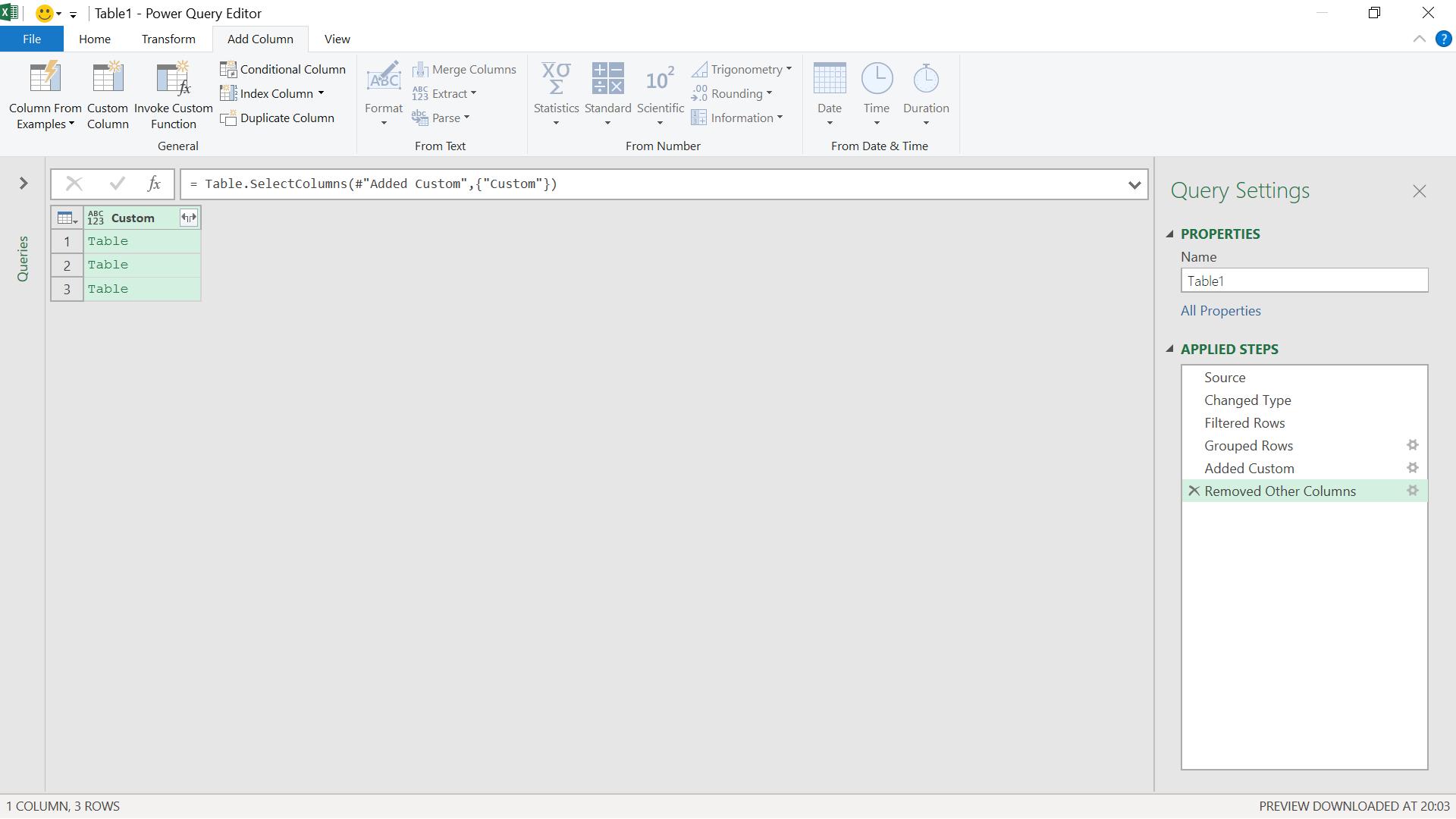
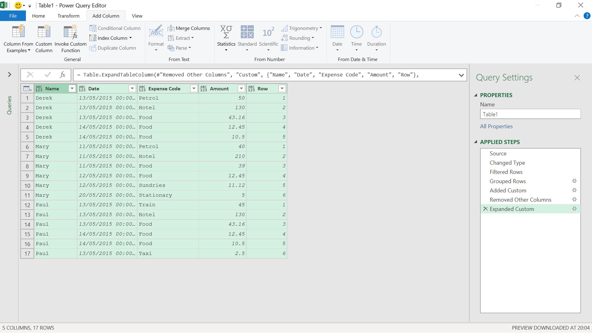
I can now expand my column.

I am almost there. I only need to show the value in Name if Row is one (1). There are several ways to do this, but I will add a ‘Conditional Column’:

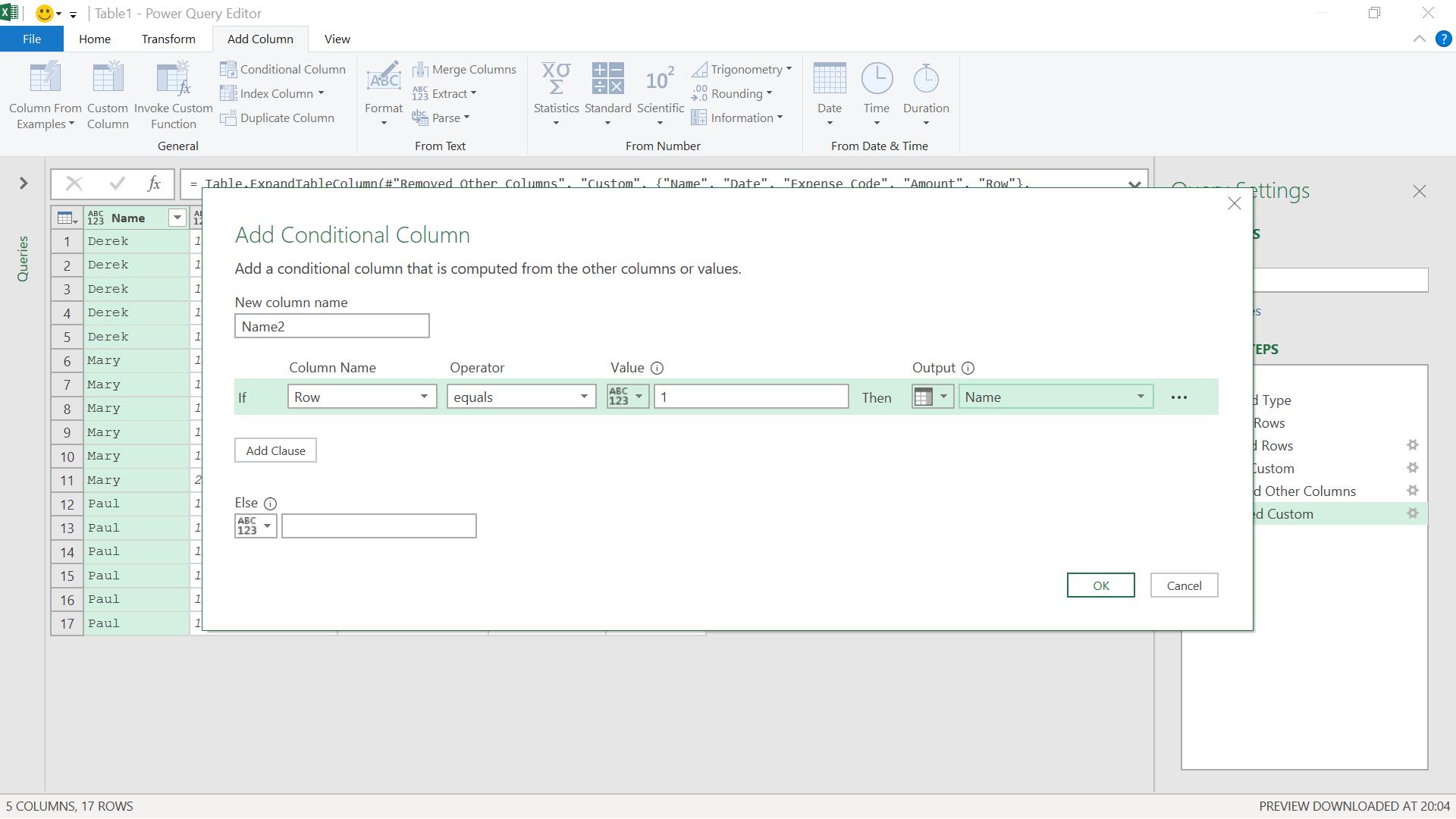
I click OK to view my data.

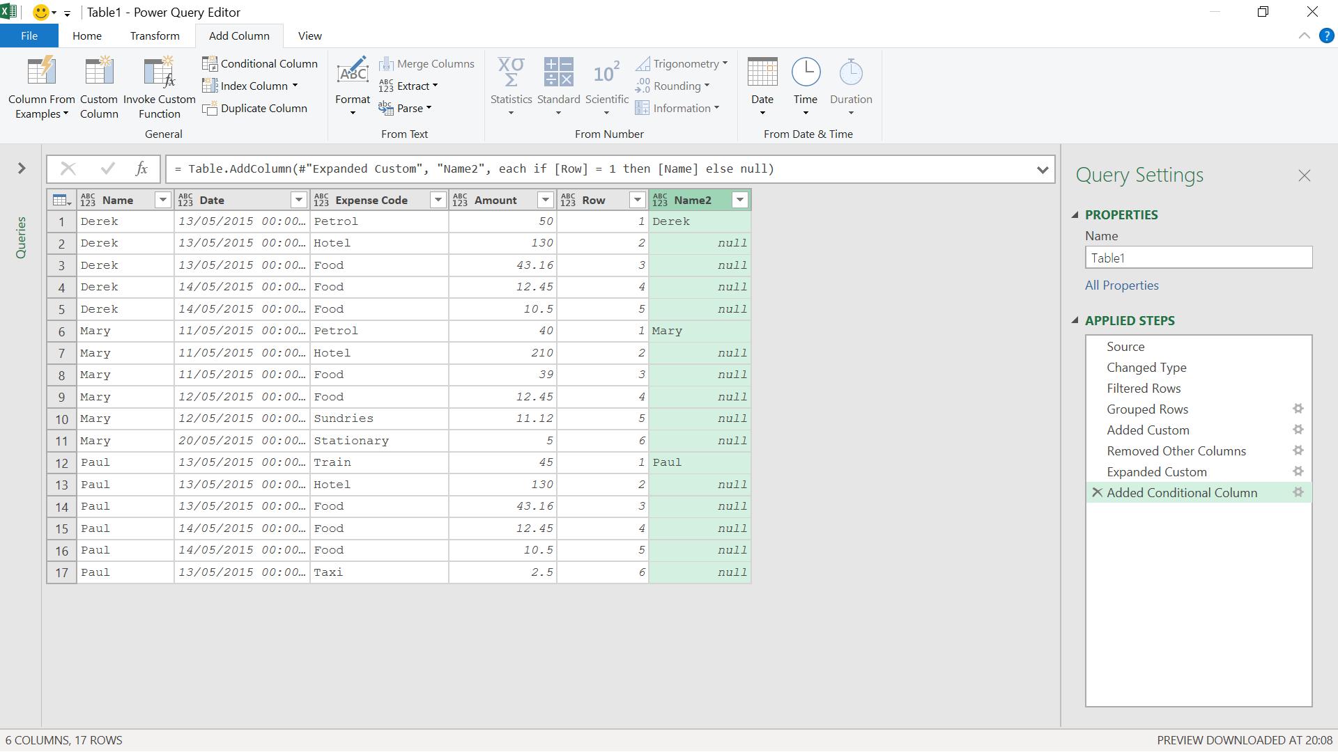
Now I can remove the original Name, rename my new column and remove the Row column I created to help me achieve my goal.

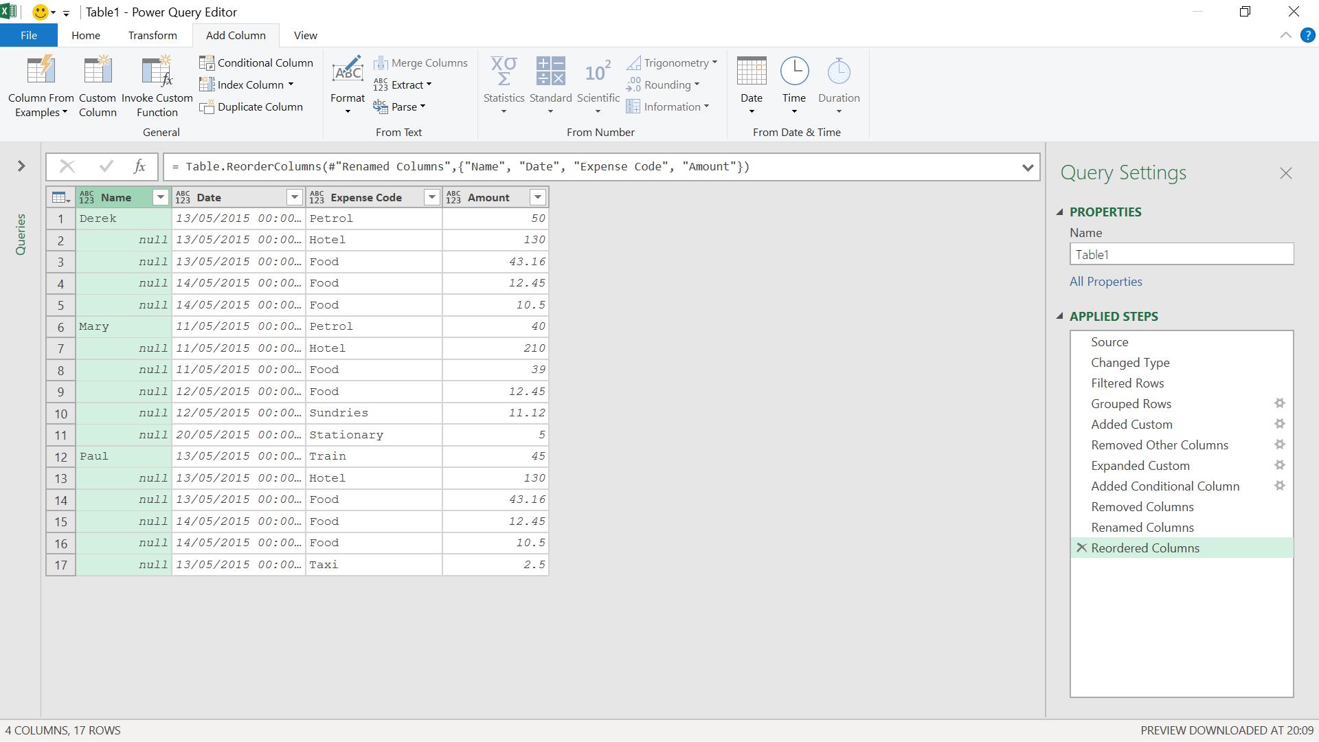
I have also reordered my columns to resemble the original table. I ‘Close & Load’ to Excel from the Home tab.

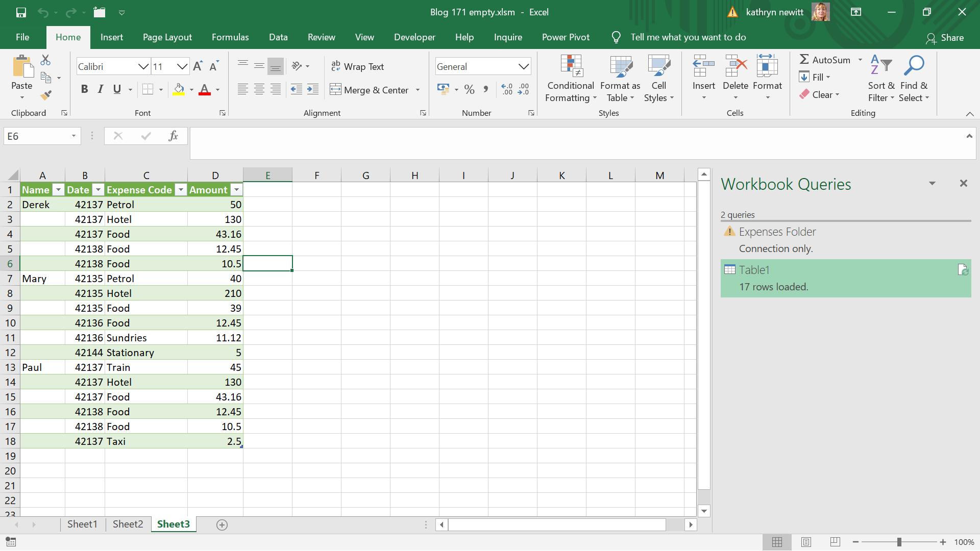
I have emptied the other cells in the column so that the data is formatted for Maureen.

Come back next time for more ways to use Power Query!