Power Query: Arranging a List

Welcome to our Power Query blog. This week, I look at how to translate a range of data contained in one cell to a list of cells.

Yet again, I have some data from my imaginary salespeople:

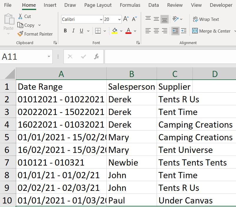
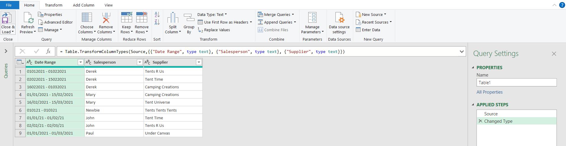
I had asked for their diary of supplier contacts, but I have instead received a list of date ranges for each salesperson and supplier. I want to have a row for each date. I start by extracting my data to Power Query using ‘From Table / Range’ on the ‘Get & Transform Data’ section of the Data tab (as usual!).

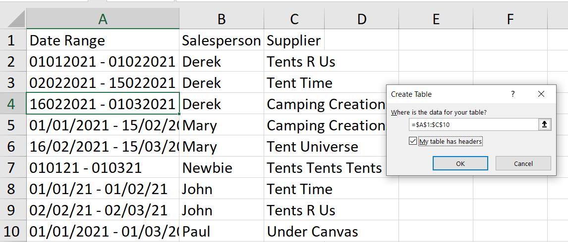
I take the default range provided in the ‘Create Table’ dialog and indicate that my data has headers.

Ultimately, I want to have a row for each date in the range. The steps I need to take in order to achieve this are:

1. Create columns for the start and end date
2. Ensure that the columns have data type date
3. Create a list of all dates between the start and end date
4. Ensure that this list is attached to the correct sales data.

In order to create the start and end date columns, I need to split Date Range by delimiter, which I can do from the Home tab.

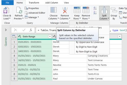
The delimiter I want to use is the dash (‘-‘).

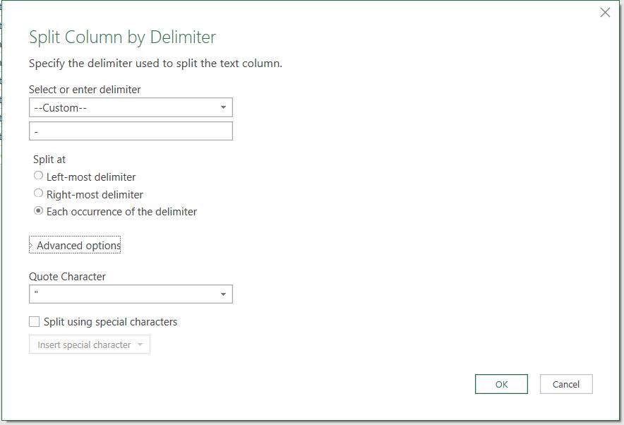
This gives me two columns which I rename Start Date and End Date for clarity.

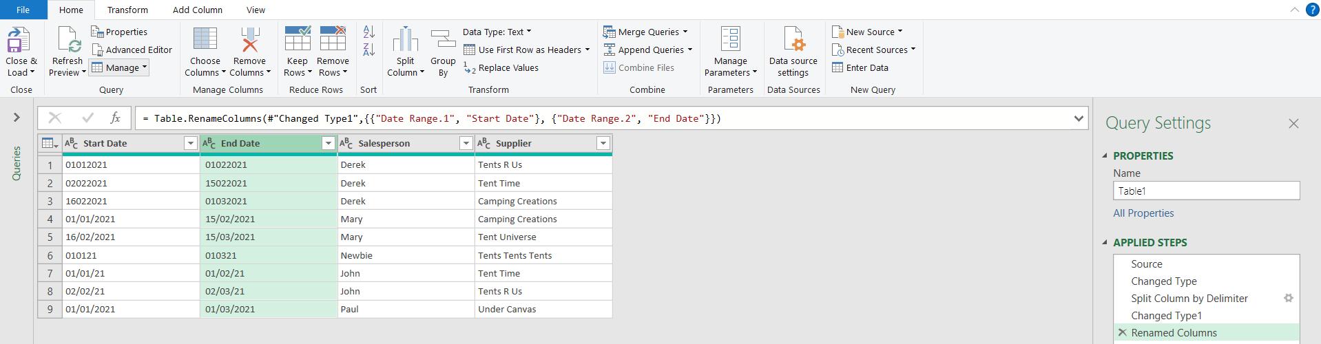
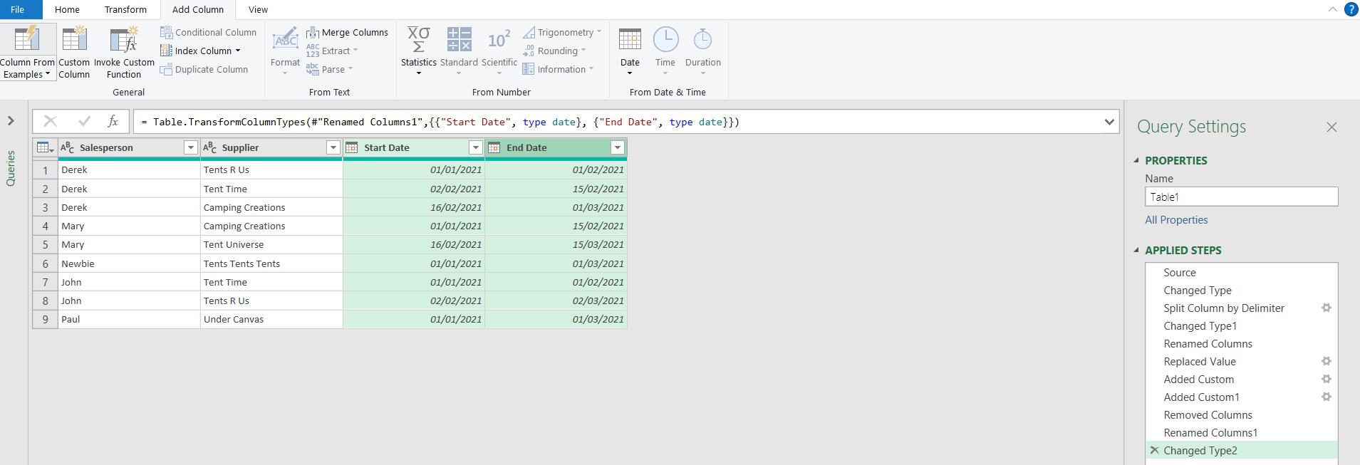
The next step is to set these columns to data type ‘Date’. I can do this in several places; I choose to select both columns and then right-click, where I can ‘Change Type’ to Date.

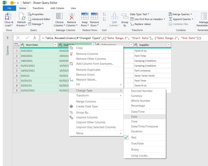
I’m hoping this copes with all the date formats used by my salespeople.

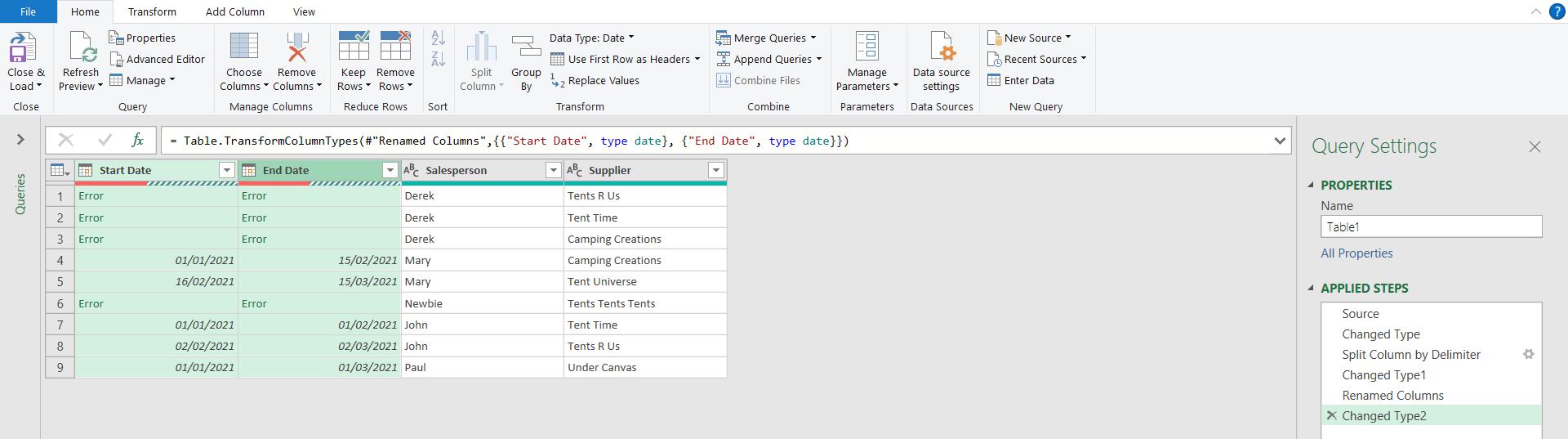
Unfortunately, this is not the case. Only the dates using a forward slash (‘/’) have been correctly converted. As I did in Power Query: Dating Options, I need to convert the columns to the format that is not being correctly formatted. I need to remove the delimiters.

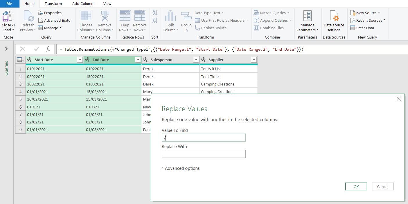
I delete the ‘Changed Type2’ step and remove all the delimiters. Next, I have to create a custom column from the ‘Add Column’ tab where I put the delimiters into each date. Although the year length varies, I am only concerned with putting a forward slash after the second and fourth characters.

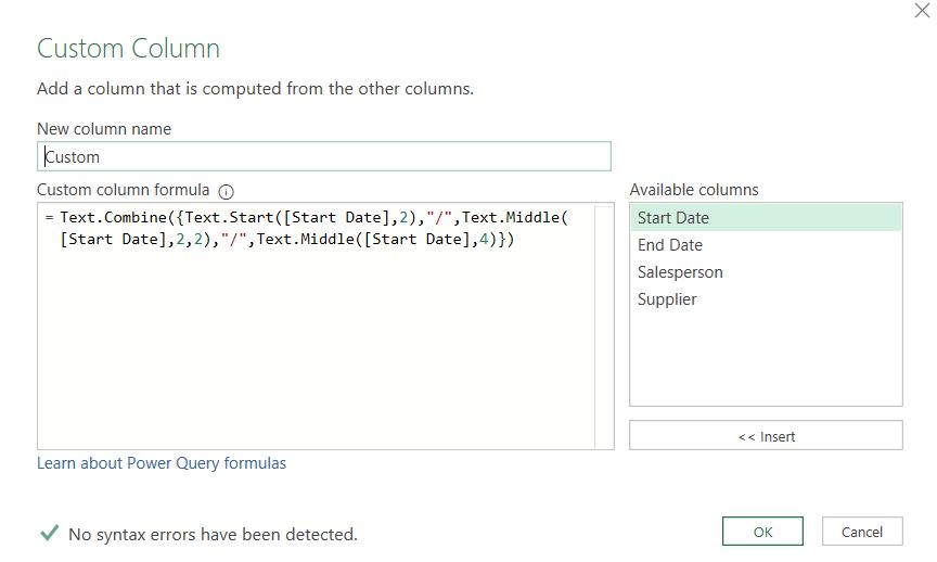
The M code I have used is:

This takes the first two characters, adds a forward slash, then adds the net two characters, adds another slash, and then adds the remaining text. Finally, the elements are combined into one text string.

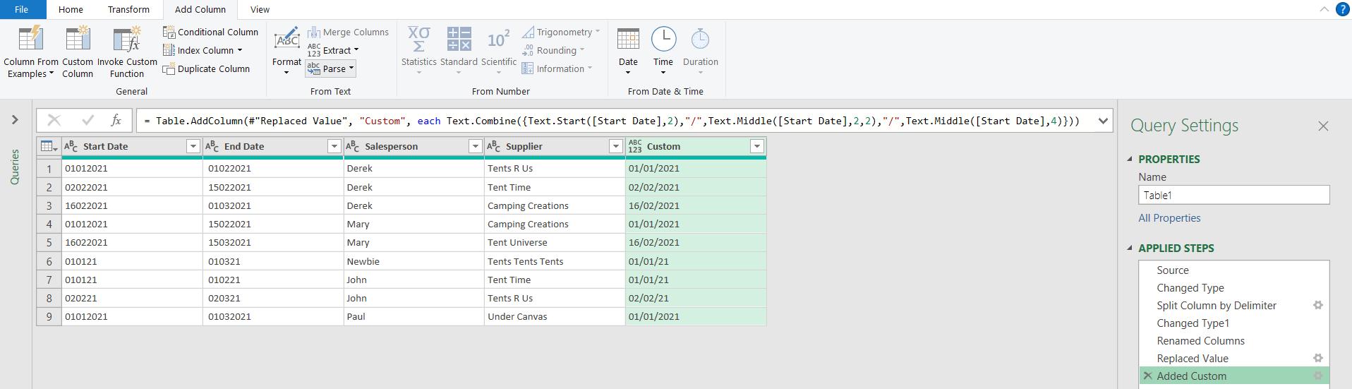
I repeat the process for the end date. Note that if there is a space at the beginning of End Date, the positions will have to be adjusted accordingly. I can then delete my original date columns and rename my new columns Start Date and End Date.

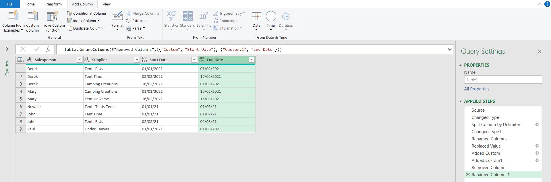
I should now be able to change the data type to ‘Date’ on my new columns.

Step 2 is complete, now I need to create a new custom column which will contain all the dates in the range. For this, I am going back to basic list creation, where I can use the ellipsis (..) to fill in the missing dates. For more on creating lists, see Power Query: Birthday Lists.

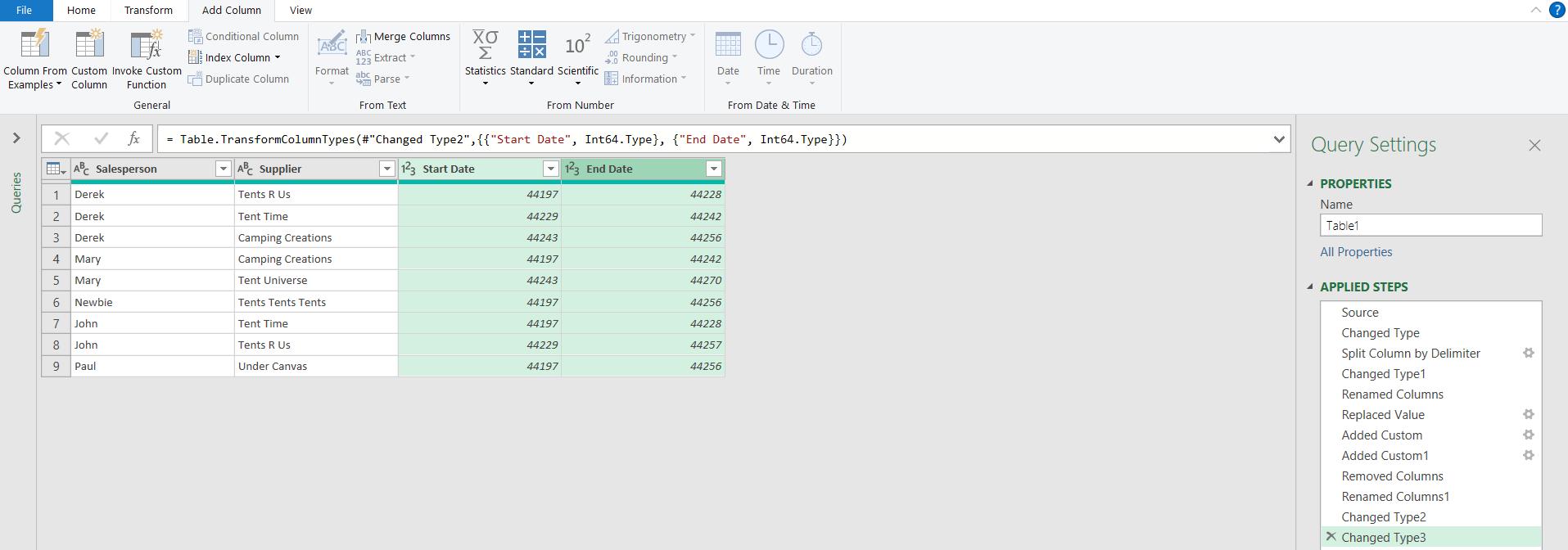
Having checked my dates are valid, I need to convert the columns to be whole numbers. This will allow me to create the list, as the ellipsis will not currently work with dates. It’s important to add a new ‘Change Type’ step for this, as I wouldn’t have been able to create a whole number from the text value with forward slashes in it.

I can now add a new custom column to create the list.

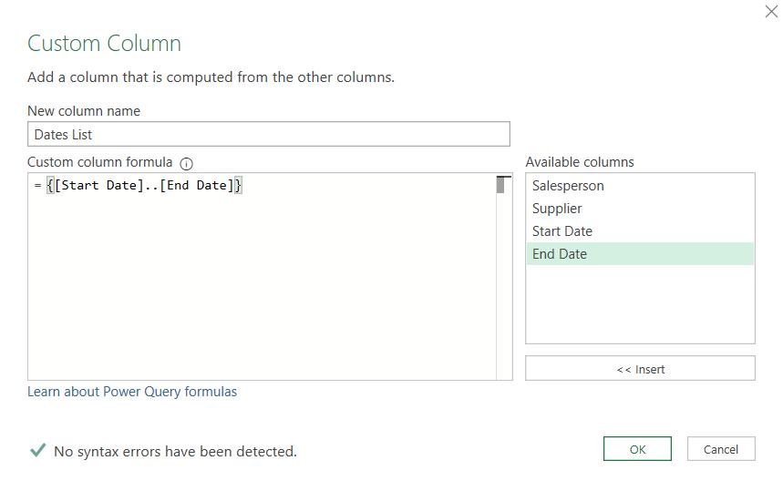
The M code I have used is:

This creates a list of numbers from Start Date to End Date, which I will be able to convert back to dates.

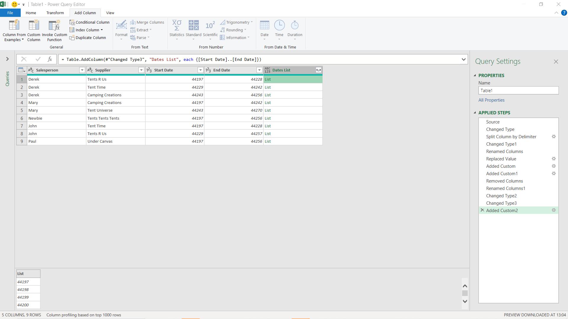
I can see that the list contains the values; now I can move to step 4, which is to expand my column.

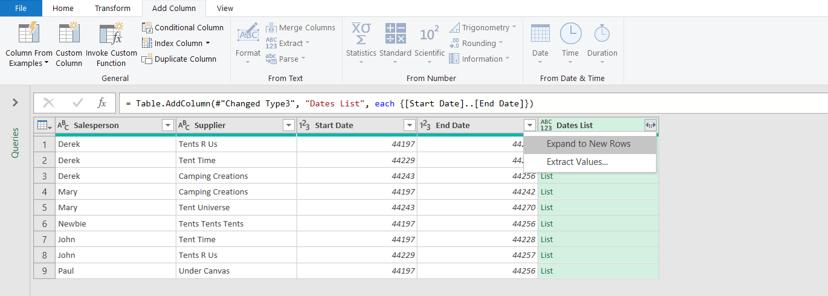
I choose to ‘Expand to New Rows’.

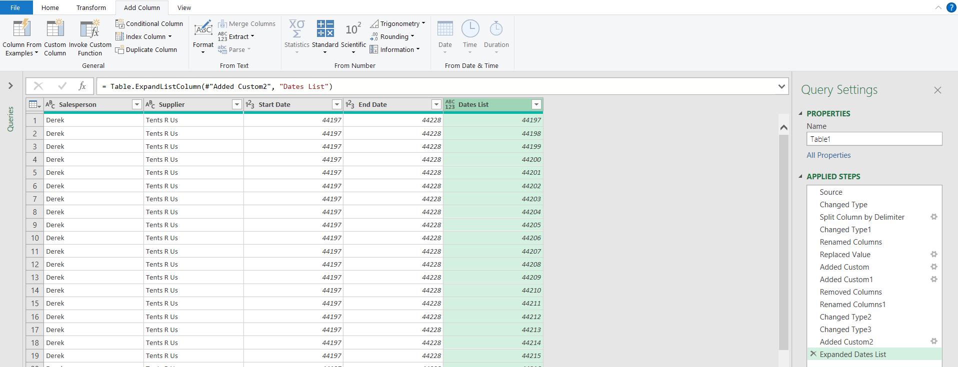
I have a row for each day. Now, I need to delete Start Date and End Date and convert Dates List to a date.

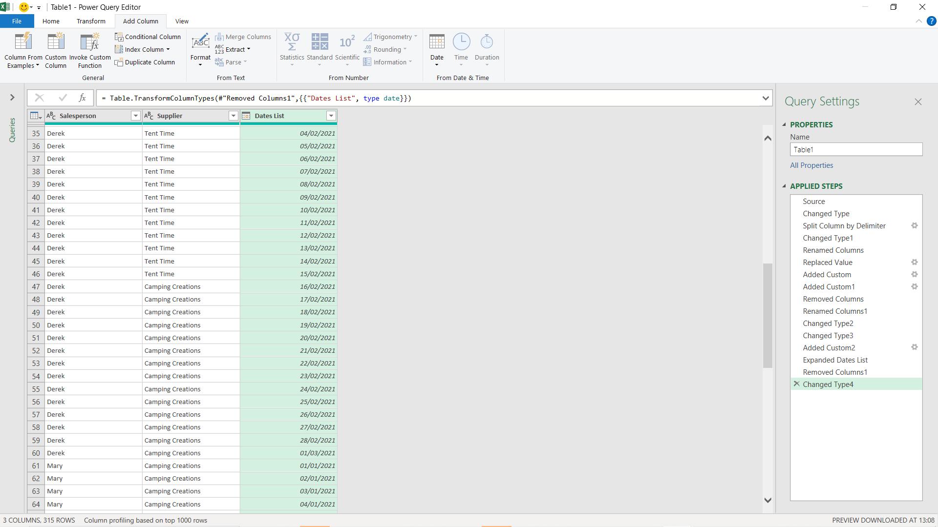
I can see that I have a row for each date with all the relevant data.

Come back next time for more ways to use Power Query!