
Power Query: Aggregating Aggravating Worksheets in Other Workbooks
3 May 2017
Welcome to our Power Query blog. Today I look at combining data from tables in Excel Worksheets in other Workbooks.
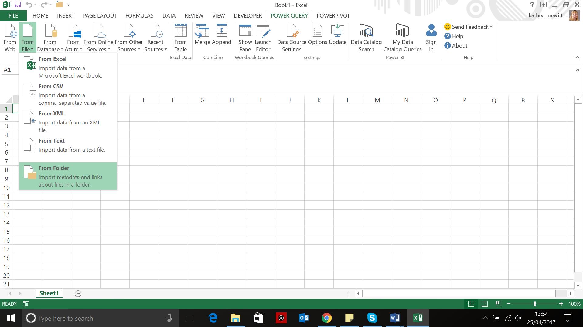
Though this may sound similar to last week’s blog, in many ways this method has just as much in common with One Folder, One Query. I will need to get a list of the workbooks that contain the data I propose to aggregate. To do this, I start in a new workbook and create a blank query which is ‘From Folder’ as shown below:
I have created a folder with my expense worksheets and some other items lurking around.
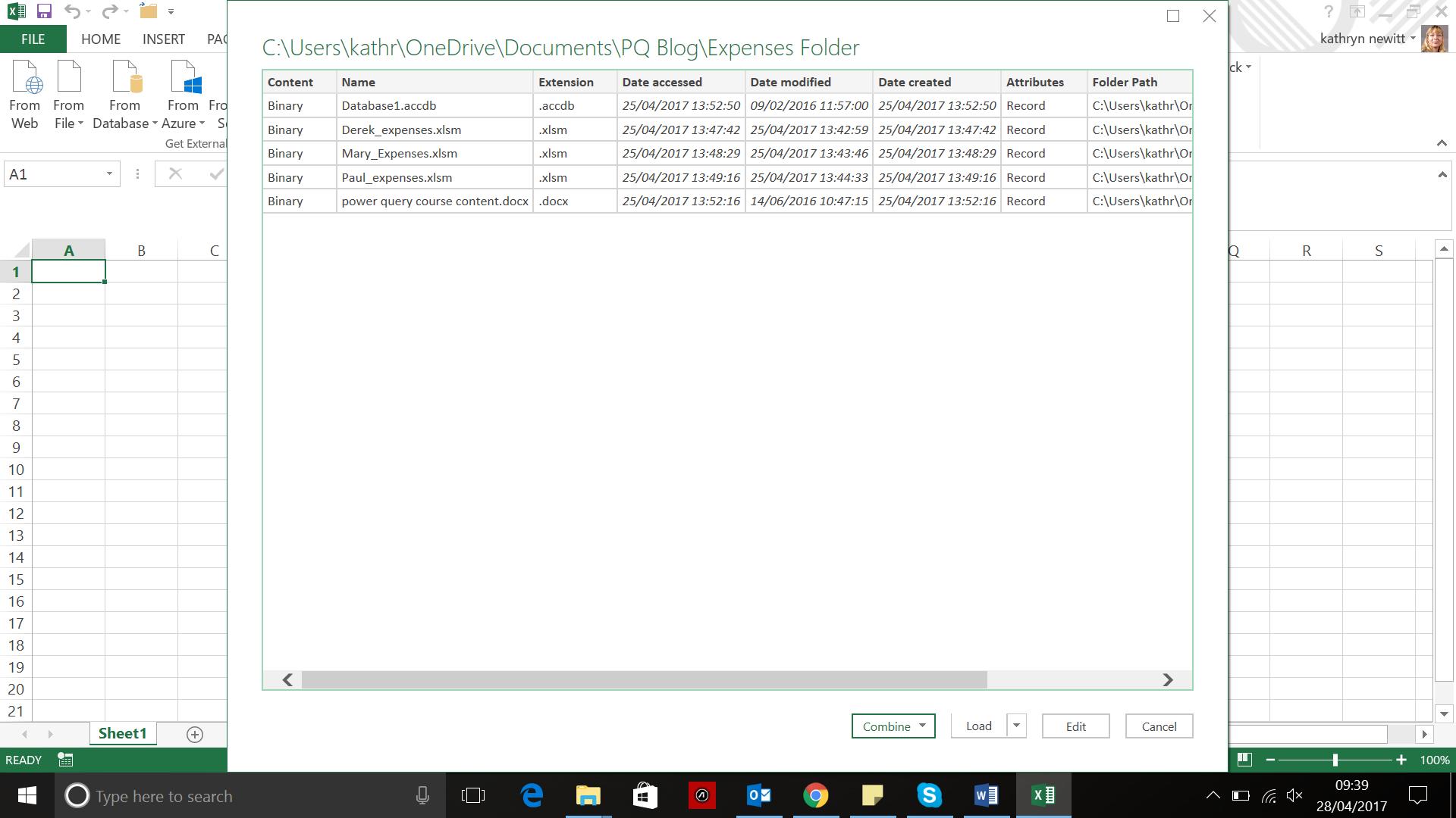
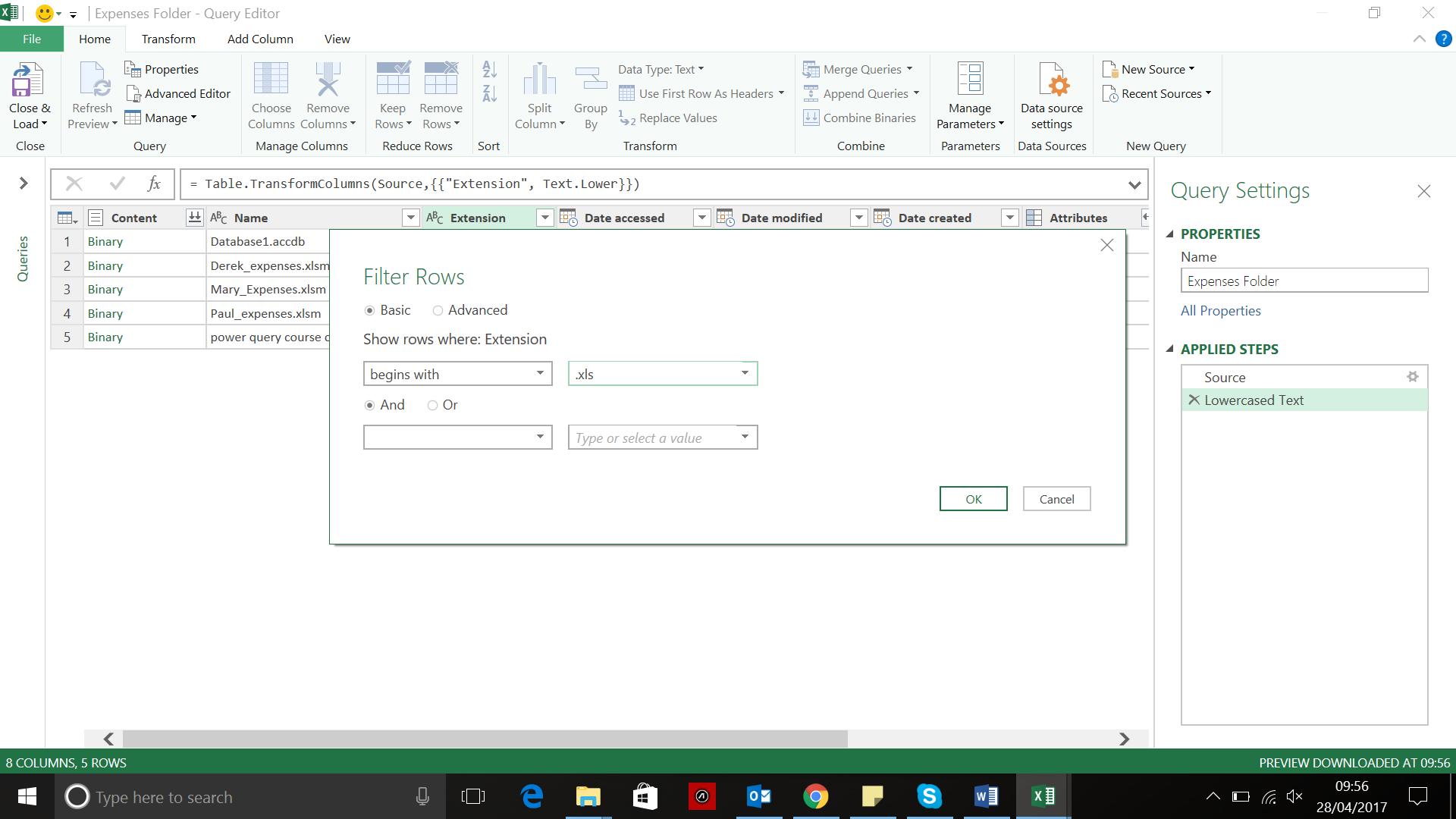
I don’t want to attempt to combine at this point as some of those files are not expenses! My next step is edit my query to filter out the other files so that I am left with the workbooks. I also want to make sure that any expense workbooks added in future would be picked up. In order that any other workbooks would also be saved regardless of the extension I transform the case to ‘lowercase’ by right-clicking on the Extension column and choosing the ‘Transform’ option. I then filter to pick up any extensions that start with ‘.xls’:
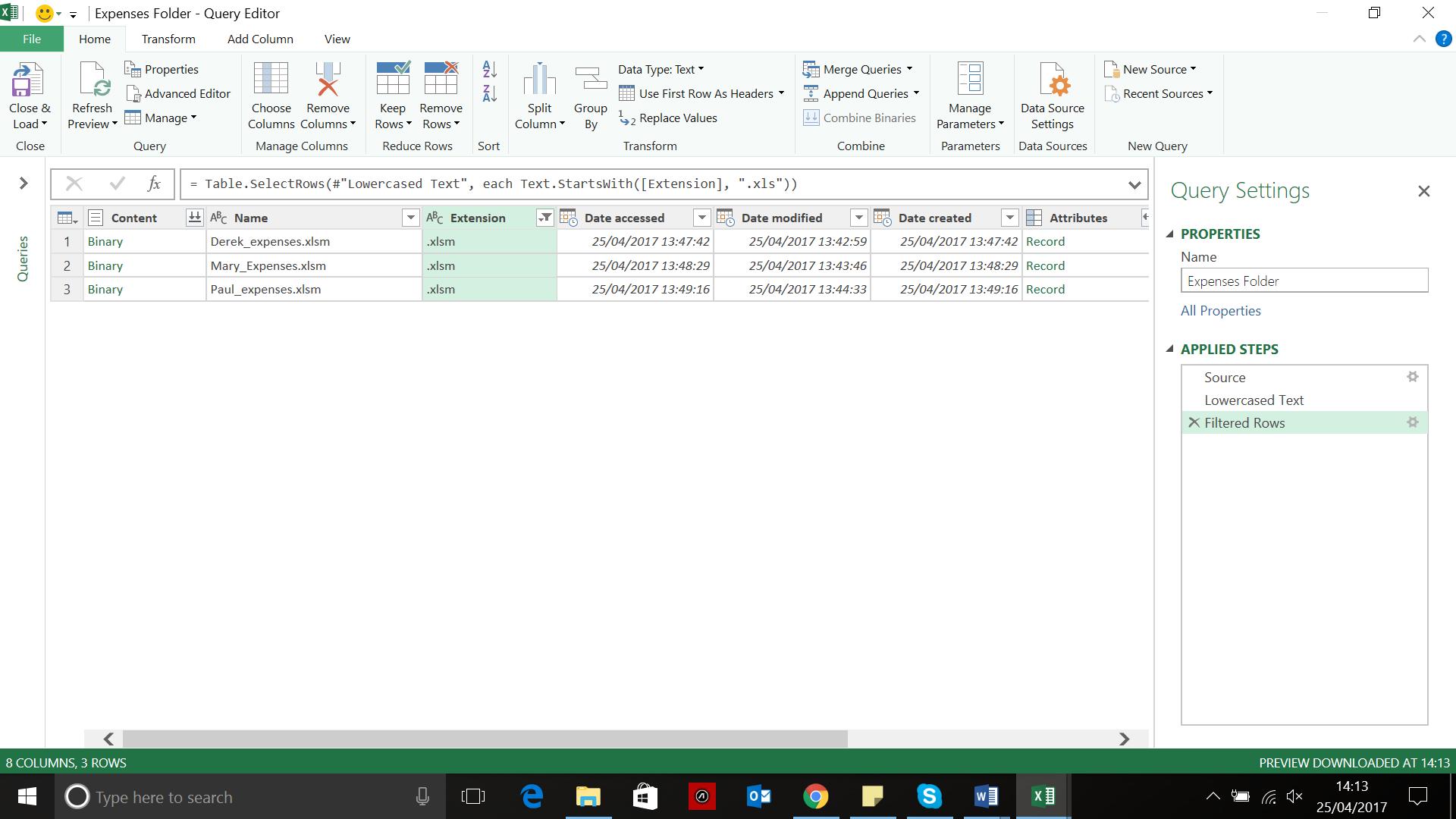
This leaves me with the files that I want.
There is an icon next to Content, since it is the ‘Combine Binaries’ button, which is tempting, so I see what it can do. Pressing it begins a process, which shows me what is available in the first file.
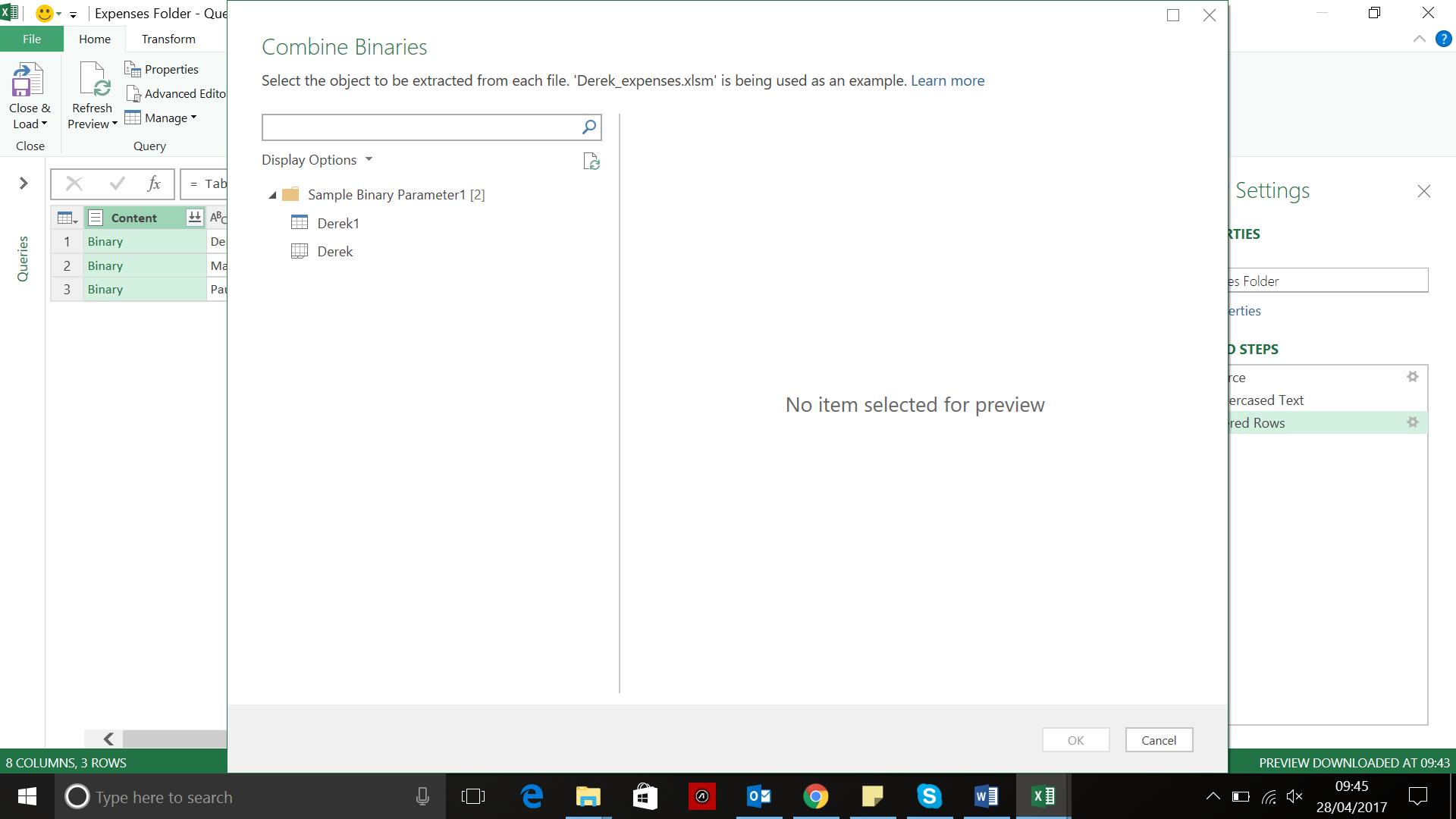
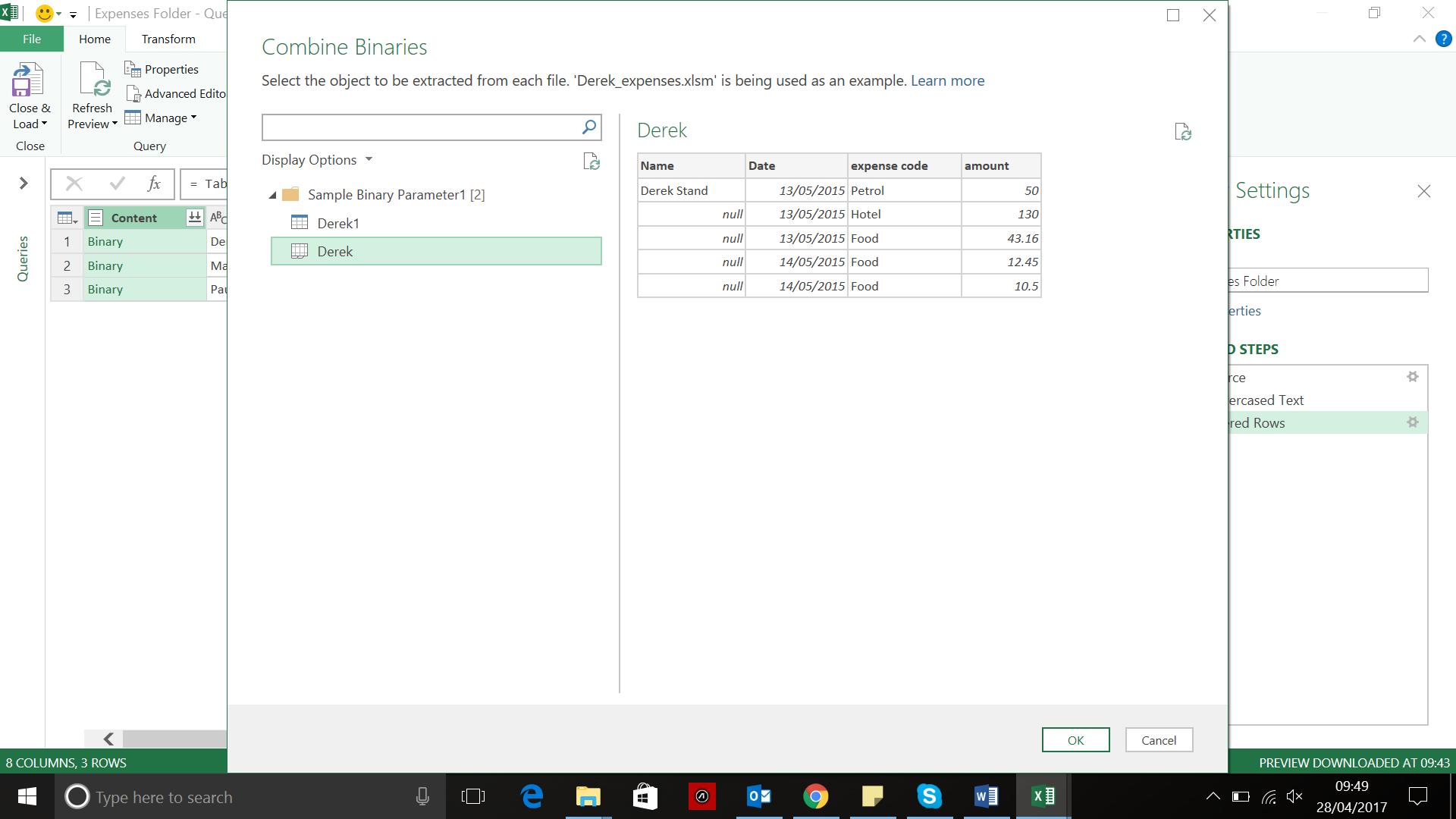
This looks promising – I have two possible icons, one that looks like a sheet, and one that looks like a table called ‘Derek1’ and ‘Derek’ respectively. When I click on them, the content looks similar. I choose the one that looks like a sheet.
I click ‘OK’ to combine the sheets.
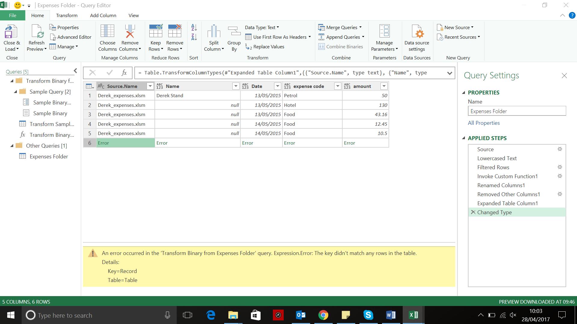
Something has gone wrong! Power Query can’t see how to link my data together, so I will need to go back to basics (the same thing happens if I were to pick the table icon instead).
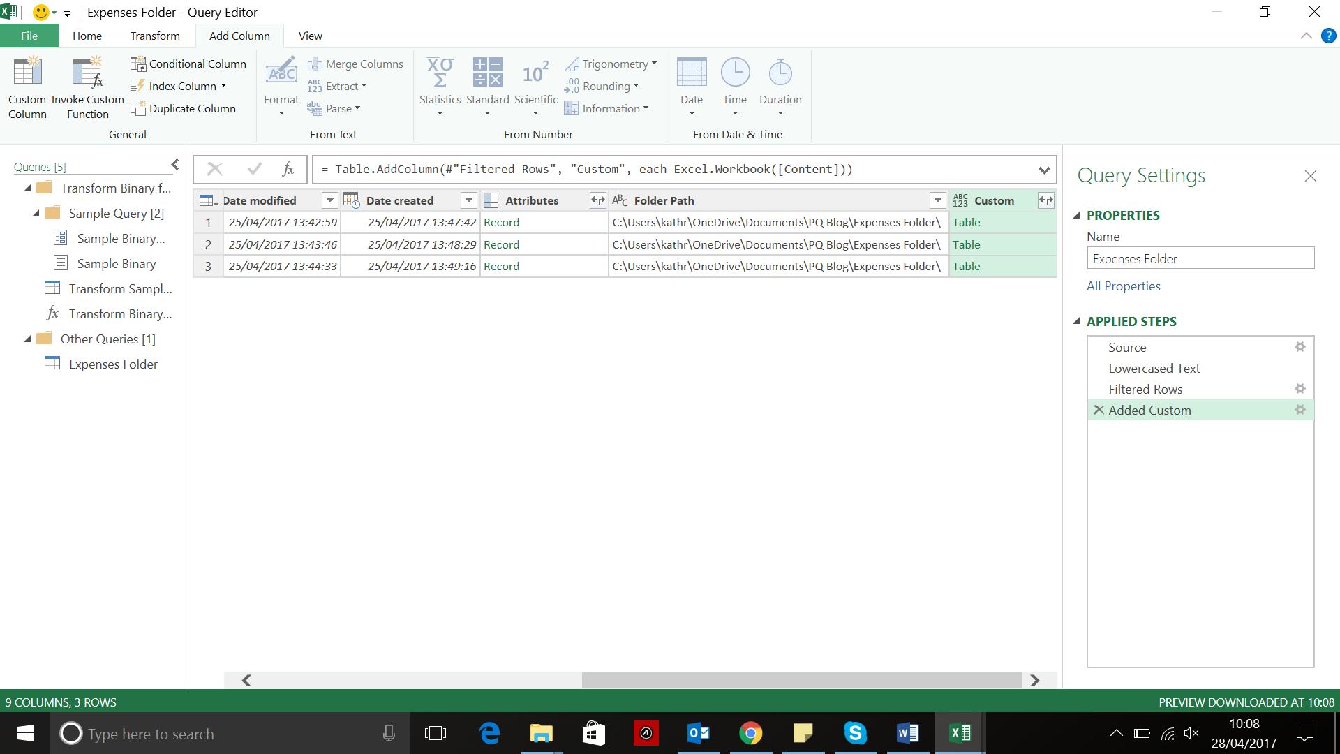
I remove the five steps that the ‘Combine Binaries’ process created, so that I am back at ‘Filtered Rows’. In the ‘Add Column’ tab I elect to add a new custom column with the following formula:
= Excel.Workbook([Content])
This should pull the Excel data from the binary content; I can also delete the content column once this is done:
My custom column promisingly contains tables, and this time the icon next to Custom can be used to expand the contents of the tables:
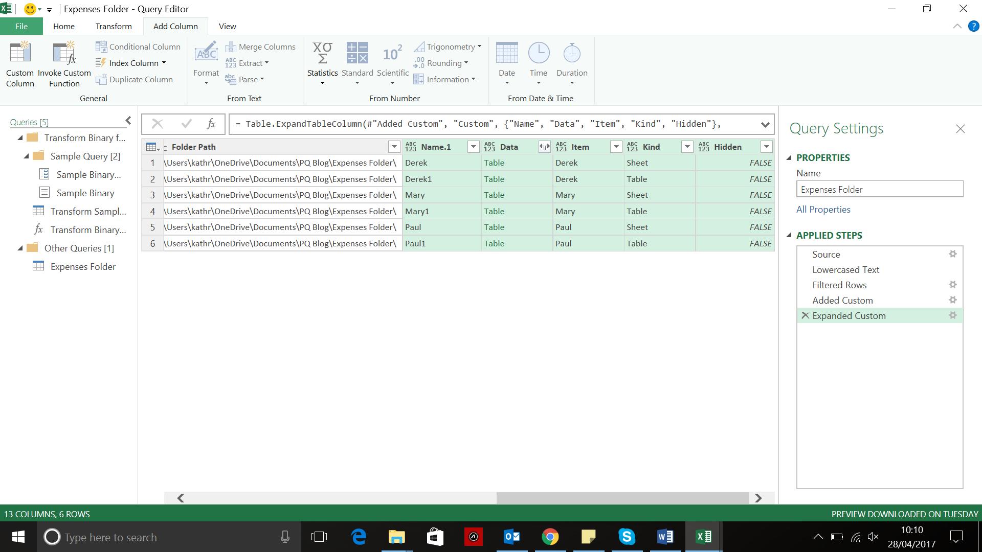
In the Kind column, I clearly have some danger of duplication as there are two rows for each person, one with value ‘Table’ and one with value ‘Sheet’. I choose to filter and keep the rows where the Kind column is populated with ‘Sheet’. I can also get rid of most of the columns as I only want the Name.1 and Data columns.
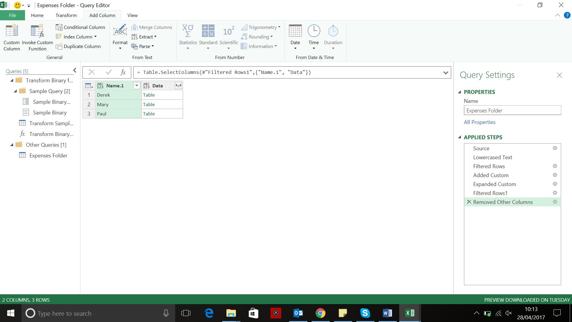
I can now expand my Data column:
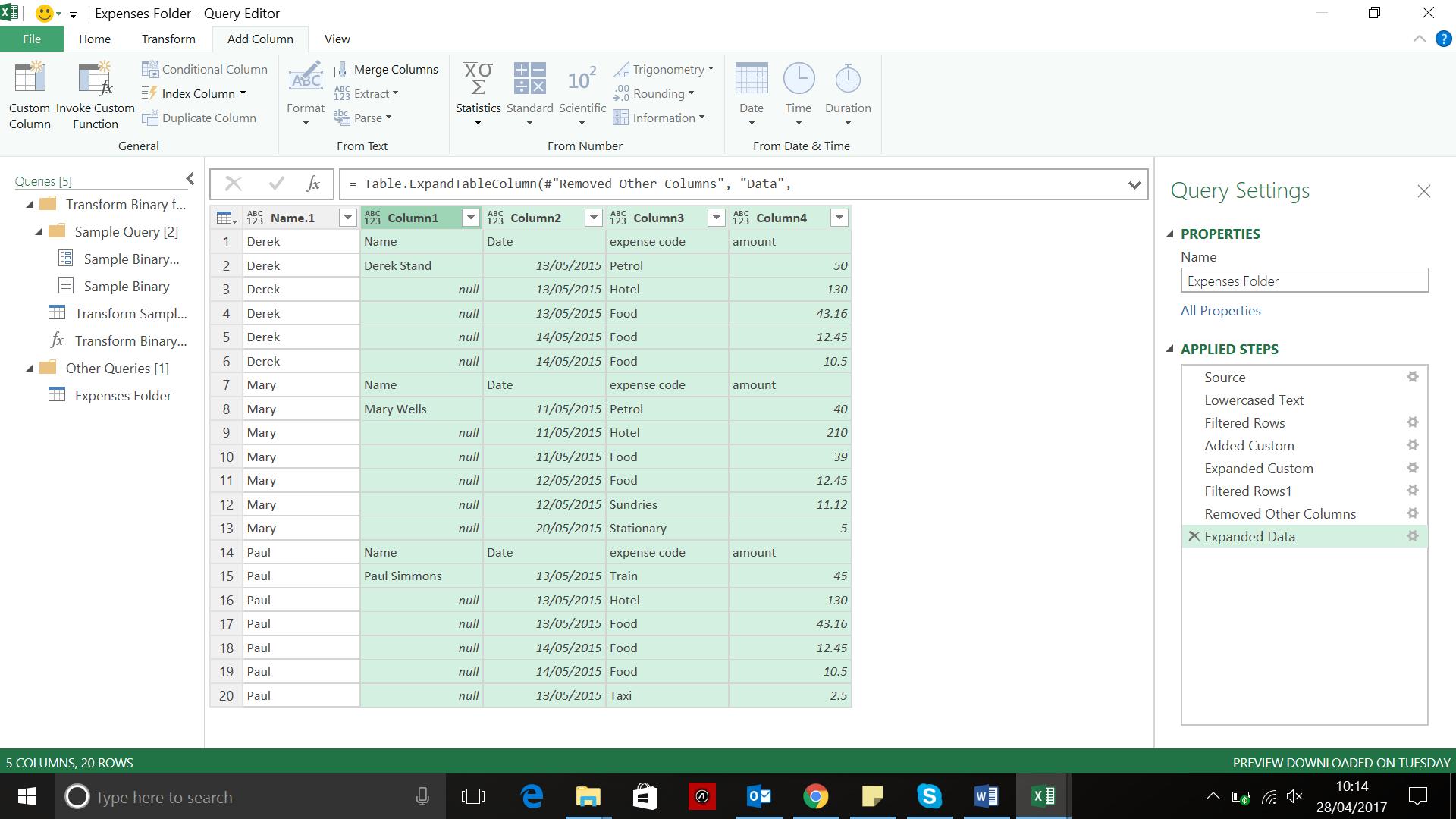
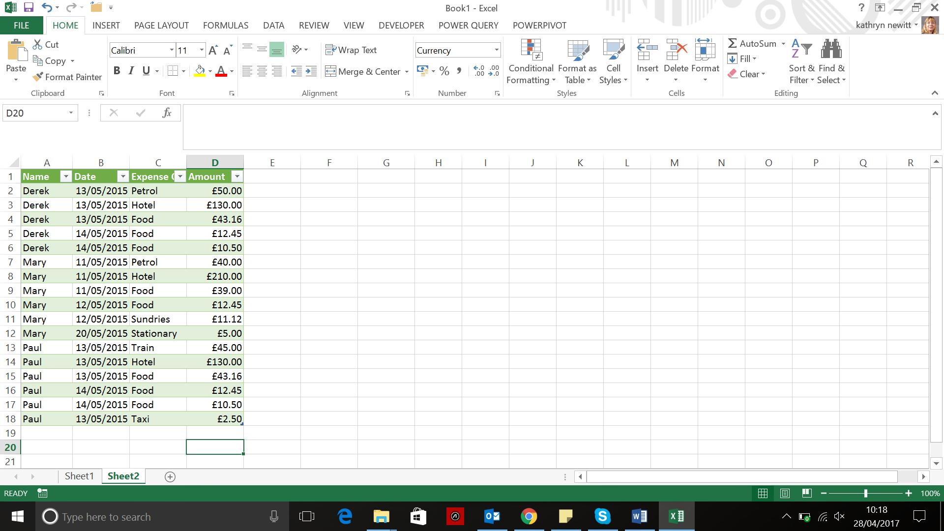
I clearly still have some tidying up to do, but the data is all there ready to be transformed. Once I am happy I can upload my data.
Want to read more about Power Query? A complete list of all our Power Query blogs can be found here. Come back next time for more ways to use Power Query!