
Power Query: Flexible Appending – Part 2
9 November 2022
Welcome to our Power Query blog. This week, I am continuing to combine data from a folder and to use a translation table to create column names.
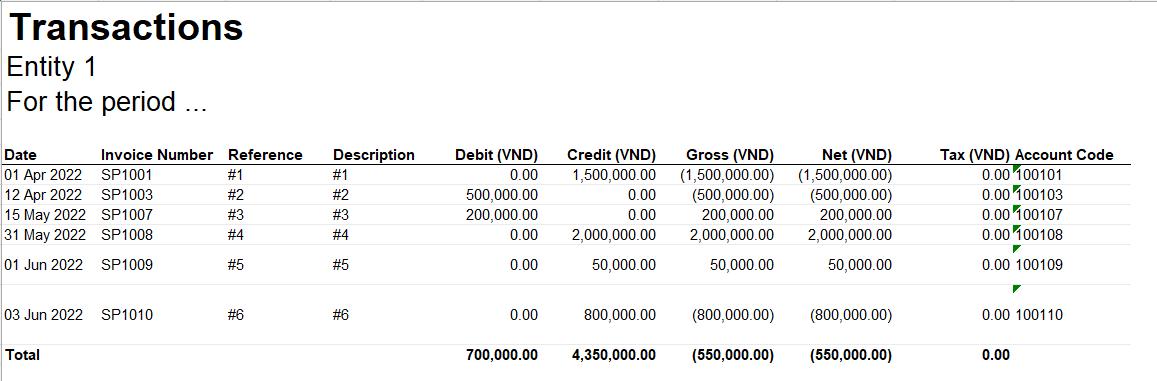
You may recall from last week I have three [3] Excel workbooks, each with some accounting data. The first file looks like this:
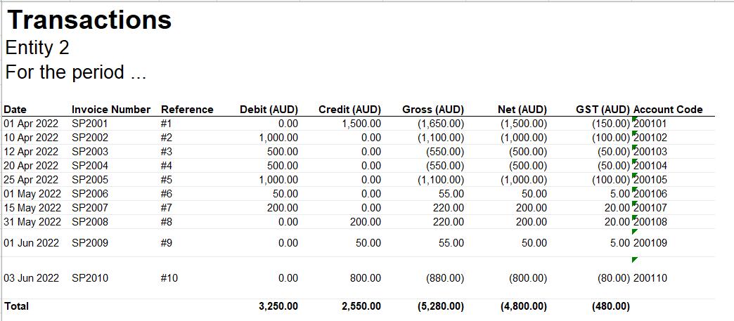
The second file looks like this:
The final file looks like this:
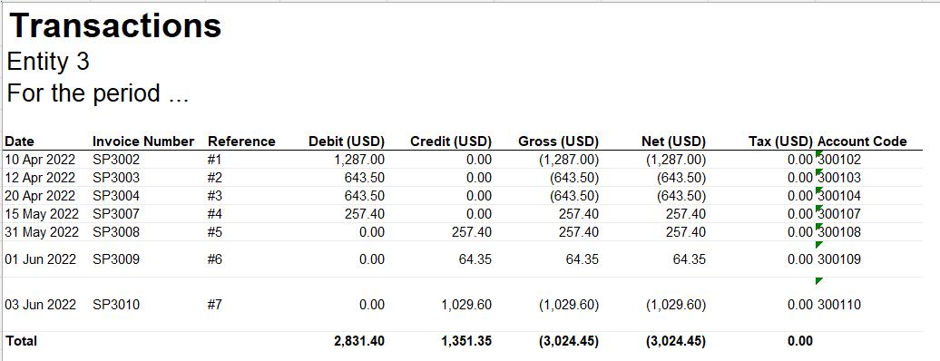
There are clearly some differences between the files. The column headings vary by country, and the first file has an extra column.
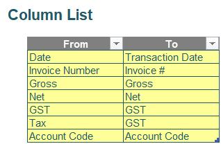
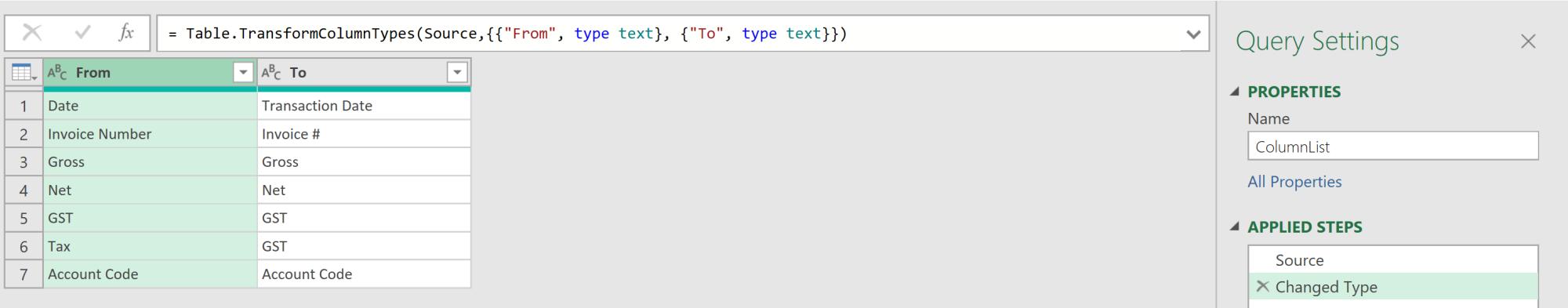
My goal is to get this data into the same table. For the purposes of this example, I am not required to convert the figures to the same currency. However, I do need to allow for more files appearing from other countries. The files are held in one folder. I have a translation table Column List in a separate Excel workbook (shown below) to help me determine the column names in the final table. No other columns are required apart from the ‘entity’ name (e.g. ‘Entity 1’).
Last week I created a query ColumnList:
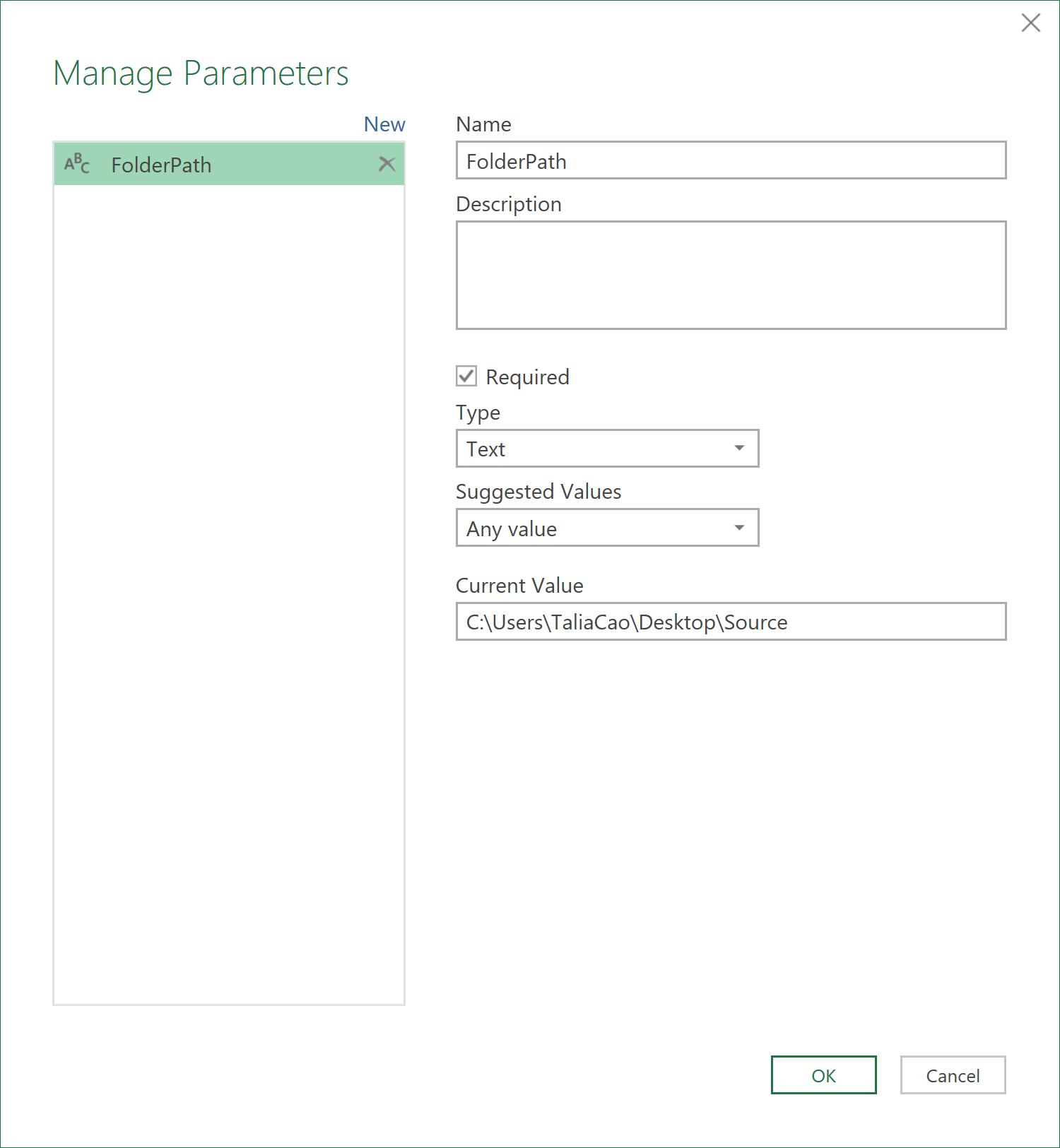
I also created a parameter called FolderPath. The ‘Current Value’ of the parameter is the folder path containing the files that I am going to append.
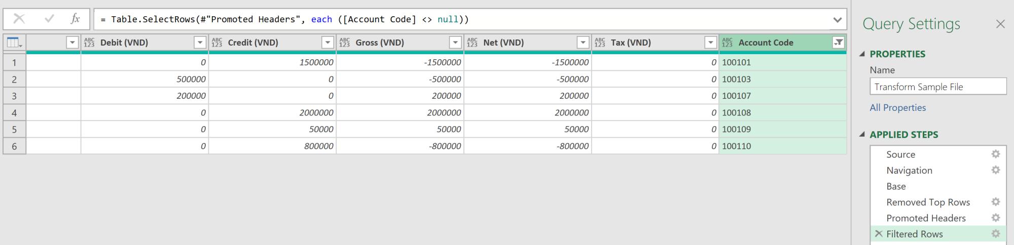
I also created and transformed a query Transform Sample File, which will act as the basis for the transformation that I need to apply to each Excel workbook in the folder.
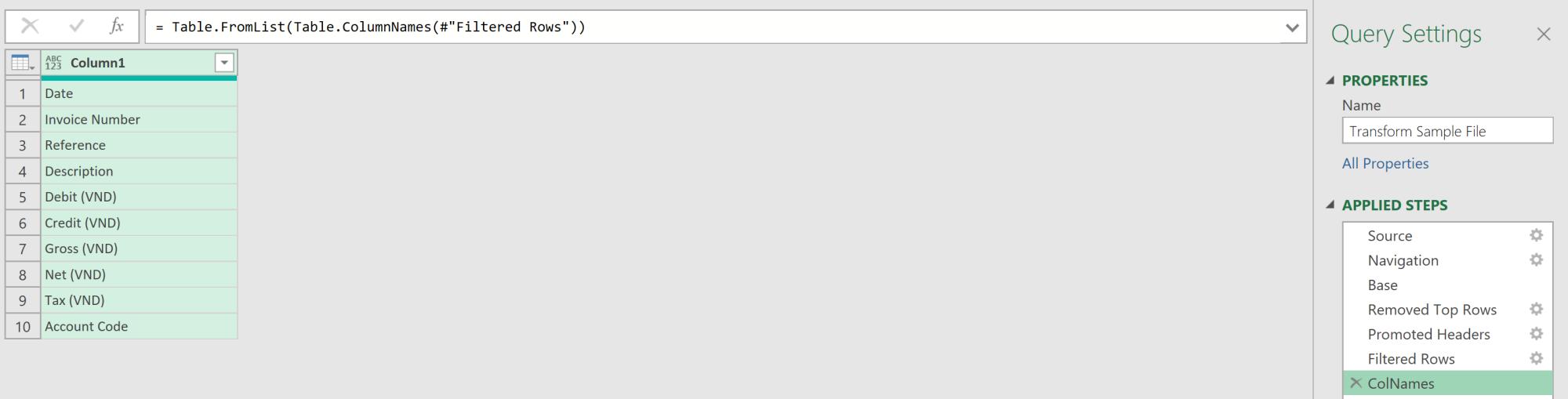
This week, I will standardise the column names. I add a new blank step with the following M code:
= Table.FromList(Table.ColumnNames(#"Filtered Rows"))
The function Table.ColumnNames() gets a list of
column names from the ‘Filtered Rows’ step and Table.FromList() then
converts that list into a table. I
rename this step to ‘ColNames’, viz.
Next, I add a custom column with the following M code:
= Table.SelectRows(ColumnList,(row) => Text.Contains([Column1], row[From]))
Table.SelectRows filters a table by a condition. The first argument is table ColumnList while the second one contains a function denoted by ‘() =>’ syntax (you should note there cannot be a space between the equals sign (=) and the greater than sign (>)).
This means that for each row in table ColumnList, Text.Contains checks whether Column1 of the current step contains the value in column From in table ColumnList. It results in a TRUE / FALSE value which is a condition for the filter.
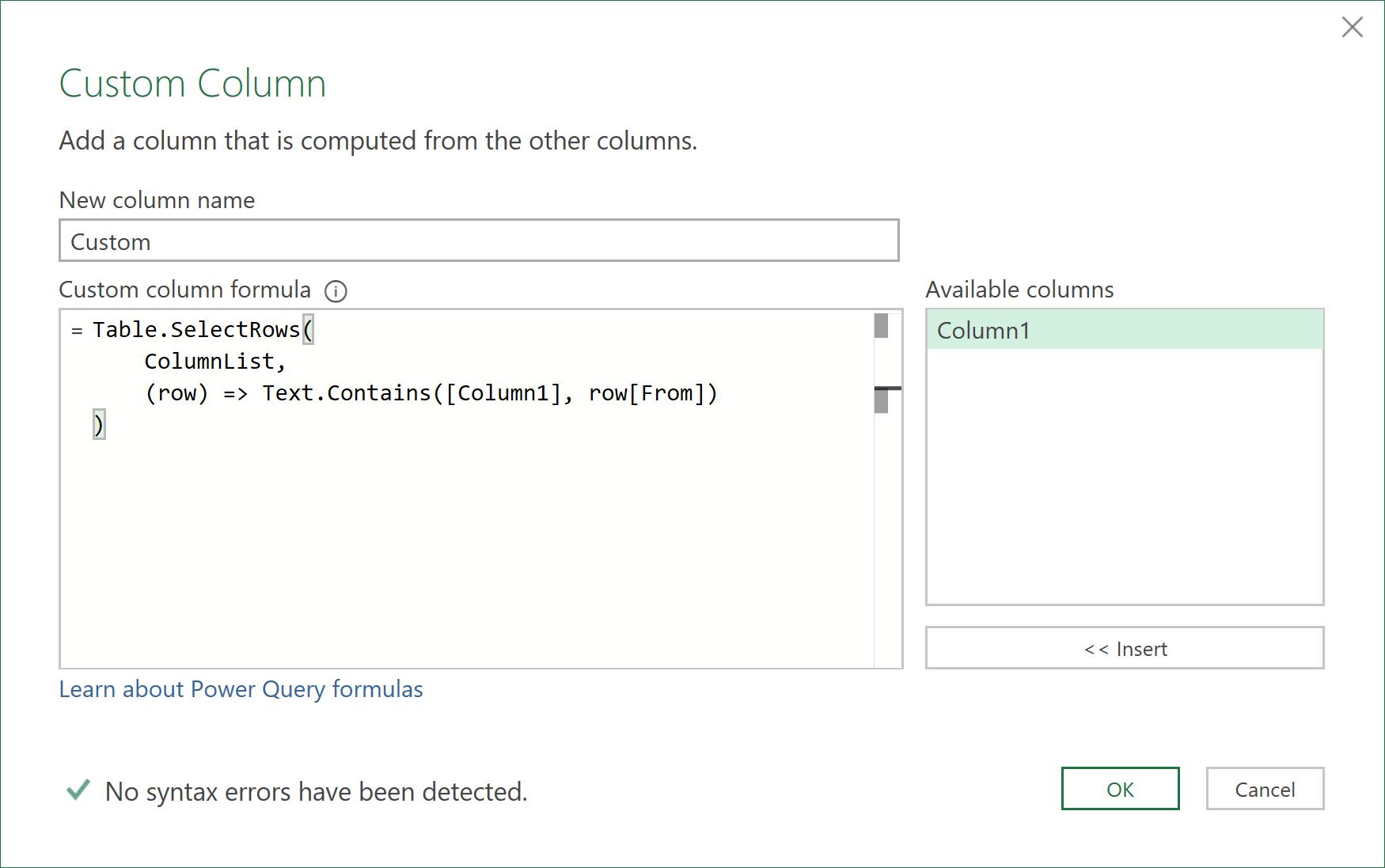
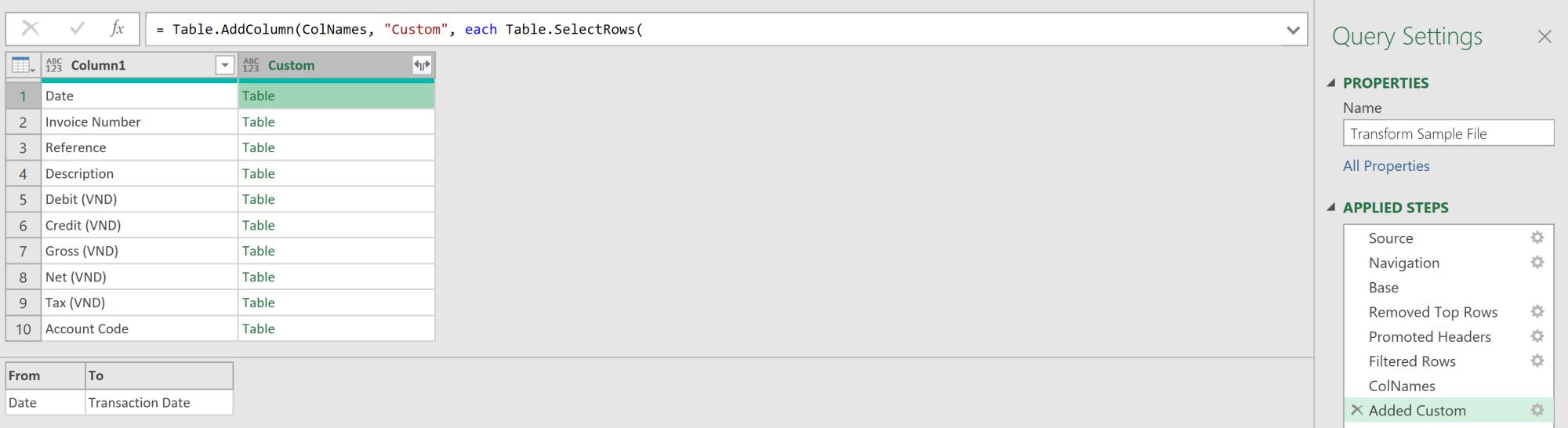
This Custom column generates tables containing rows that meet the condition.
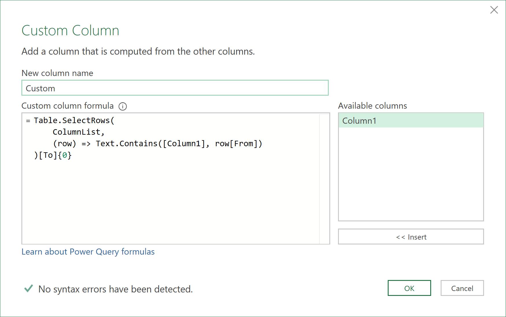
Within these tables, I would like to get the first value of column To by adding “[To]{0}” to the end of the M code.
Table.SelectRows( ColumnList, (row) => Text.Contains([Column1], row[From]) )[To]{0}
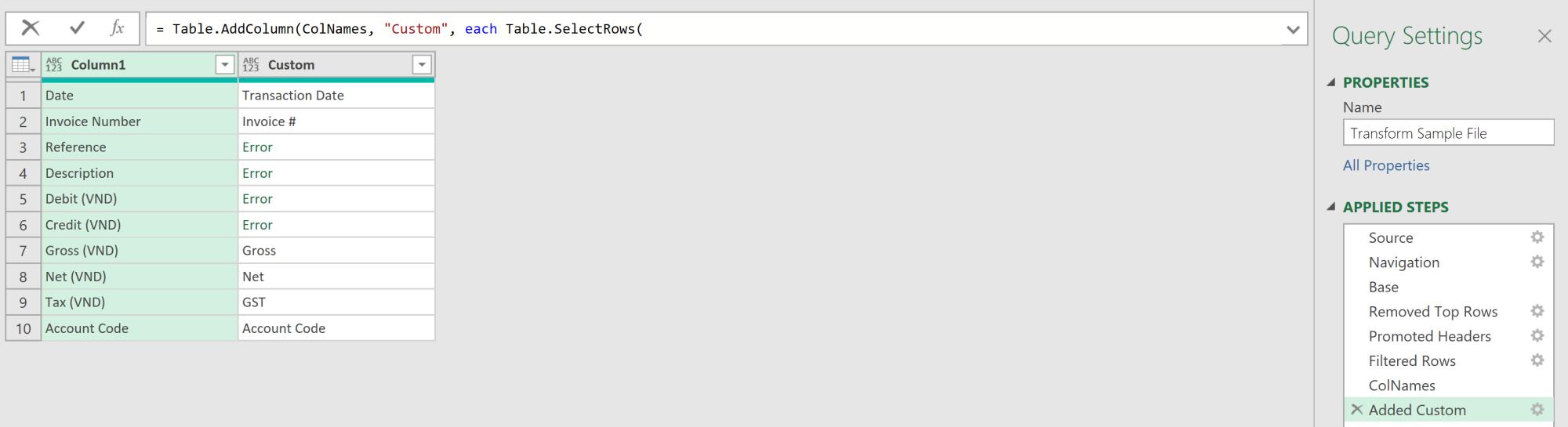
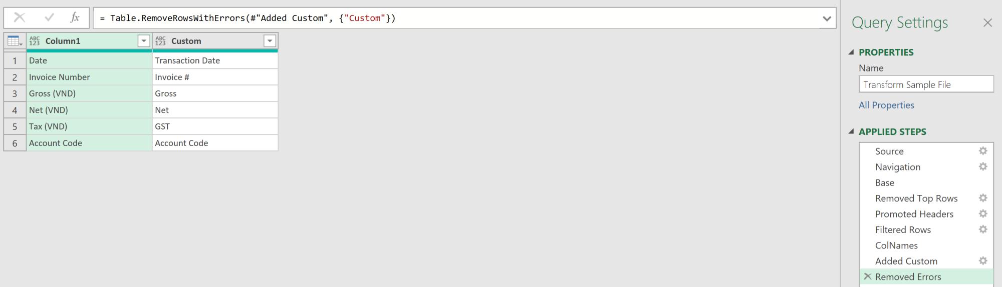
There are some errors for those columns which have no matches from ColumnList. I don’t need these columns, so I right-click and apply ‘Remove Errors’ to the Custom column, which means I am left with a list of columns I want to keep without hardcoding any column names.
Next time, I will complete the example by applying the list of from and to values to each of the extracted Excel sheets.
Come back next time for more ways to use Power Query!