
Power Pivot Principles: Introducing the REMOVEFILTERS Function in DAX
20 October 2020
Welcome back to the Power Pivot Principles blog. This week, we will talk about the REMOVEFILTERS function in DAX.
The REMOVEFILTERS function clears filters from the tables or columns specified. This function has the following syntax:
REMOVEFILTERS([table|column[, column[, column[,…]]]])
In DAX, the filter removal functionality already exists in another function which is the ALL function. Compared to the ALL function, the REMOVEFILTERS function is also fairly straightforward, but they do differ. The REMOVEFILTERS function can only be used to clear filters, rather than return a table. In contrast, the ALL function returns the table or column with the filters removed.
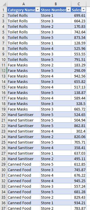
Let’s consider an example. Imagine you have a Sales data set, with four product categories in five stores, which has already been loaded into the Power Pivot Data Model. We want to get the percentage of sales by each category or by each store.
In the Power Pivot Data Model, we create the Sales Amount and Total Sales measures:
Sales Amount:=SUM([Sales])
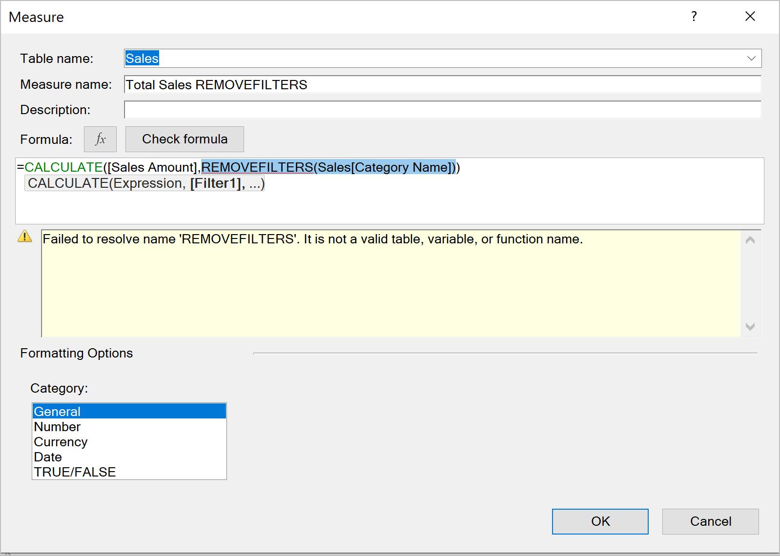
Total Sales REMOVEFILTERS:=CALCULATE([Sales Amount],REMOVEFILTERS(Sales[Category Name])
However, the following error appears: the REMOVEFILTERS function is not yet available in Power Pivot!
For this instance, we will need to illustrate our example in Power BI Desktop. We will load the data from the Excel file into Power BI Desktop. Next, we need to create the Sales Amount and Total Sales measures:
Sales Amount = SUM([Sales])
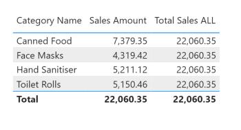
Total Sales ALL = CALCULATE([Sales Amount],ALL(Sales[Category Name]))
Then, if we replace the ALL function with the REMOVEFILTERS function:
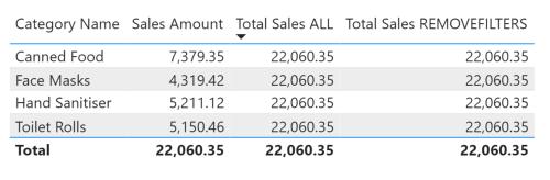
Total Sales REMOVEFILTERS = CALCULATE([Sales Amount], REMOVEFILTERS(Sales[Category Name]))
It will give us the same result.
We can also remove filters from multiple columns, from the whole table, or the entire data model.
Total Sales REMOVEFILTERS = CALCULATE([Sales Amount], REMOVEFILTERS(Sales[Category Name],Sales[Store Number]))
Total Sales REMOVEFILTERS = CALCULATE([Sales Amount], REMOVEFILTERS(Sales))
Total Sales REMOVEFILTERS = CALCULATE([Sales Amount], REMOVEFILTERS())
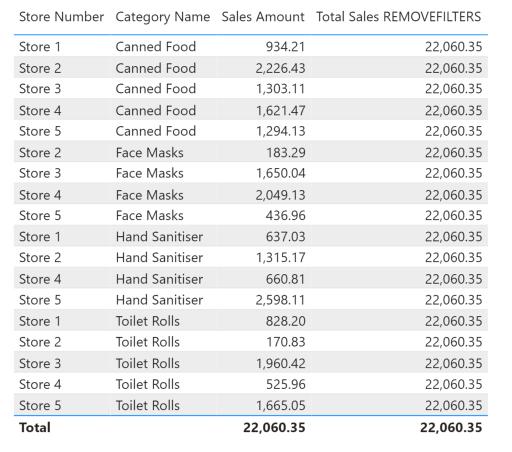
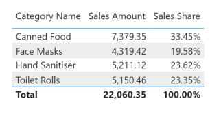
Therefore, we can create the Sales Share measure to get percentage of sales by category:
Sales Share = DIVIDE([Sales Amount], [Total Sales REMOVEFILTERS])
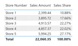
If we remove the Category Name from the table and drag the Store Number to replace it, the measure still calculates correctly:
This function was announced in the Power BI Desktop updates in September 2019. Now that it has been a year, hopefully it will appear in Power Pivot soon…
That’s it for this week!
Stay tuned for our next post on Power Pivot in the Blog section. In the meantime, please remember we have training in Power Pivot which you can find out more about here. If you wish to catch up on past articles in the meantime, you can find all of our Past Power Pivot blogs here.