
Power Pivot Principles: Introduction to Key Performance Indicators (KPIs) in Power Pivot
10 November 2020
Welcome back to the Power Pivot Principles blog. So far, we have discussed only about using measures in Power Pivot. This week, we will move away from measures and talk about Key Performance Indicators (KPIs).
A Key Performance Indicator (KPI) is a quantifiable measurement for gauging business objectives e.g. measuring sales performance against target sales, comparing actual figures versus budget. A KPI includes a base value, a target value and status thresholds:
- a base value is a calculated field that must result in a value, for example, can be an aggregate of sales or the profit for a specific period
- a target value is also a calculated field that results in a value, being a measure or an absolute value. For instance, a sales manager wishes to see how each department is performing, where the budget calculated field would represent the target value
- a status threshold is defined by the range between a low and high threshold, which displays with a graphic to help users easily determine the status of the base value compared to the target value.
Let’s consider an example on how to create a KPI in Power Pivot, using a SalesData table, by stores and by product types in the first quarter of FY20/21, which has already been loaded into the Power Pivot Data Model:
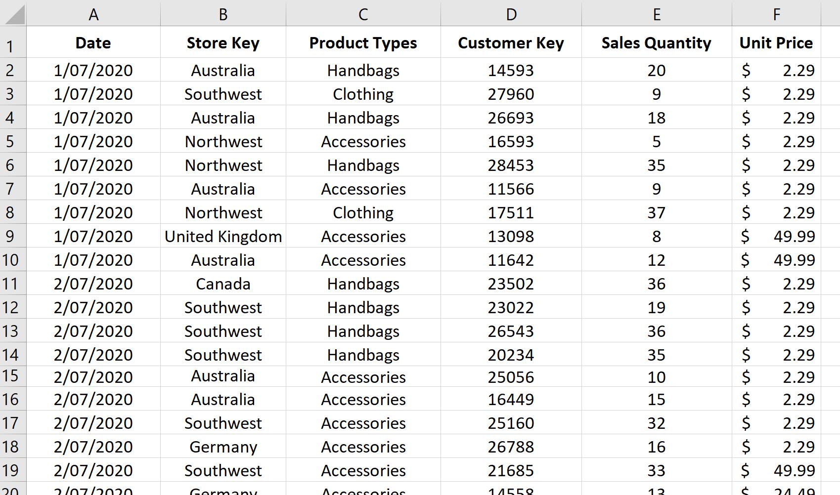
We will create a measure to get sales which will be the base value, from which we will create the KPI later:
Total Sales:=SUMX(Sales,Sales[Sales Quantity]*Sales[Unit Price])
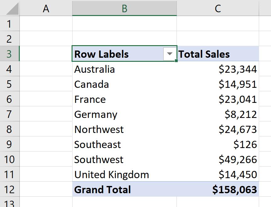
We will create a PivotTable to see Total Sales by Store Key:
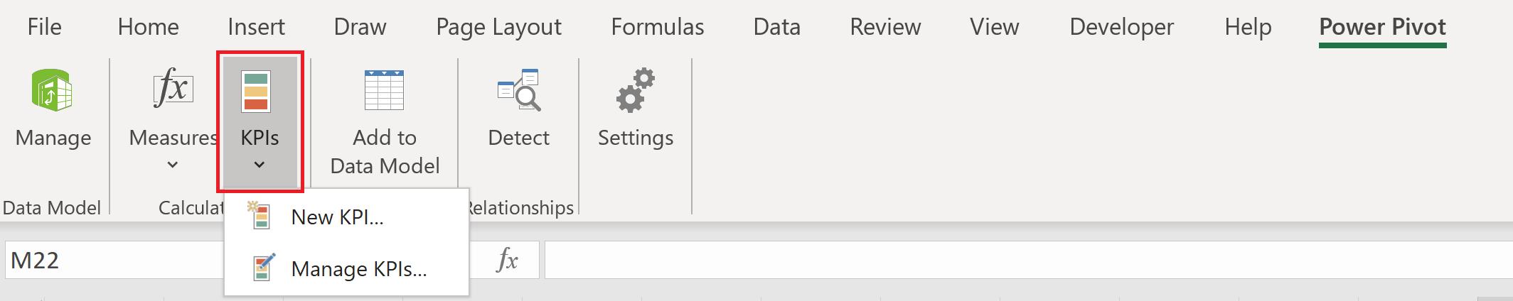
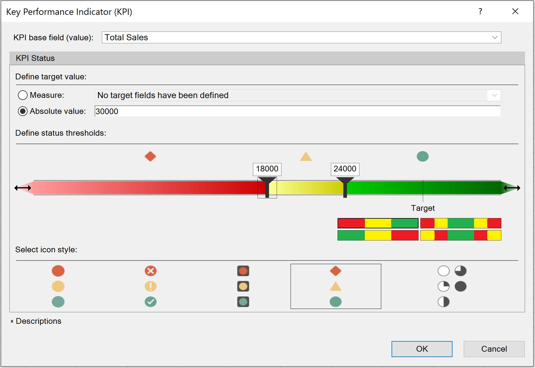
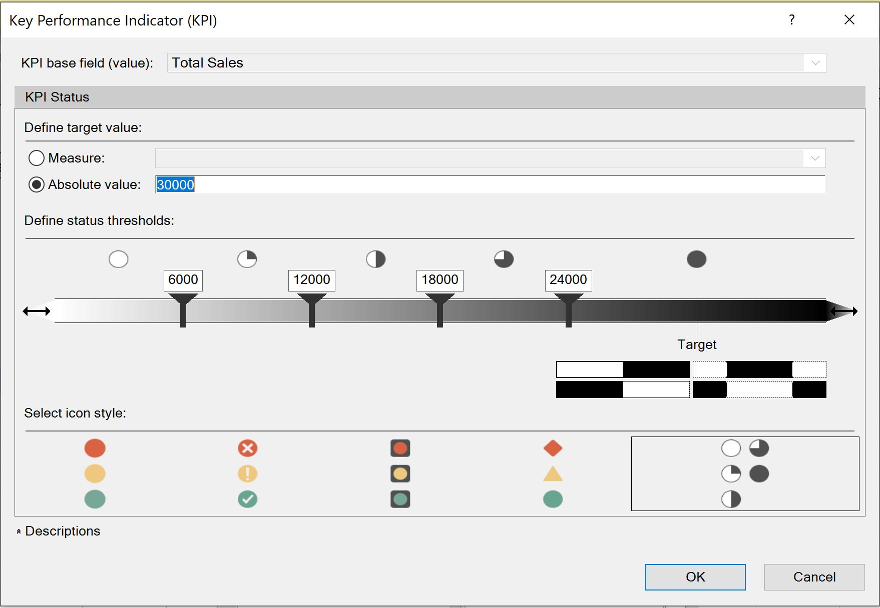
Now, we want to see how each store performs against a sales target, by creating a KPI. We navigate to the ‘Power Pivot’ tab on the Ribbon, choose KPIs -> New KPI…, where a Key Performance Indicator (KPI) dialog will appear. We will select Total Sales as the ‘KPI base field (value)’ and in the ‘Define target value’ section, we will enter an ‘Absolute value’ of 30,000. We can also select the icon style and adjust the status threshold, e.g. a red icon for Total Sales below $18,000, yellow for Total Sales between $18,000 and $24,000, and a green one for stores with Total Sales of over $24,000:
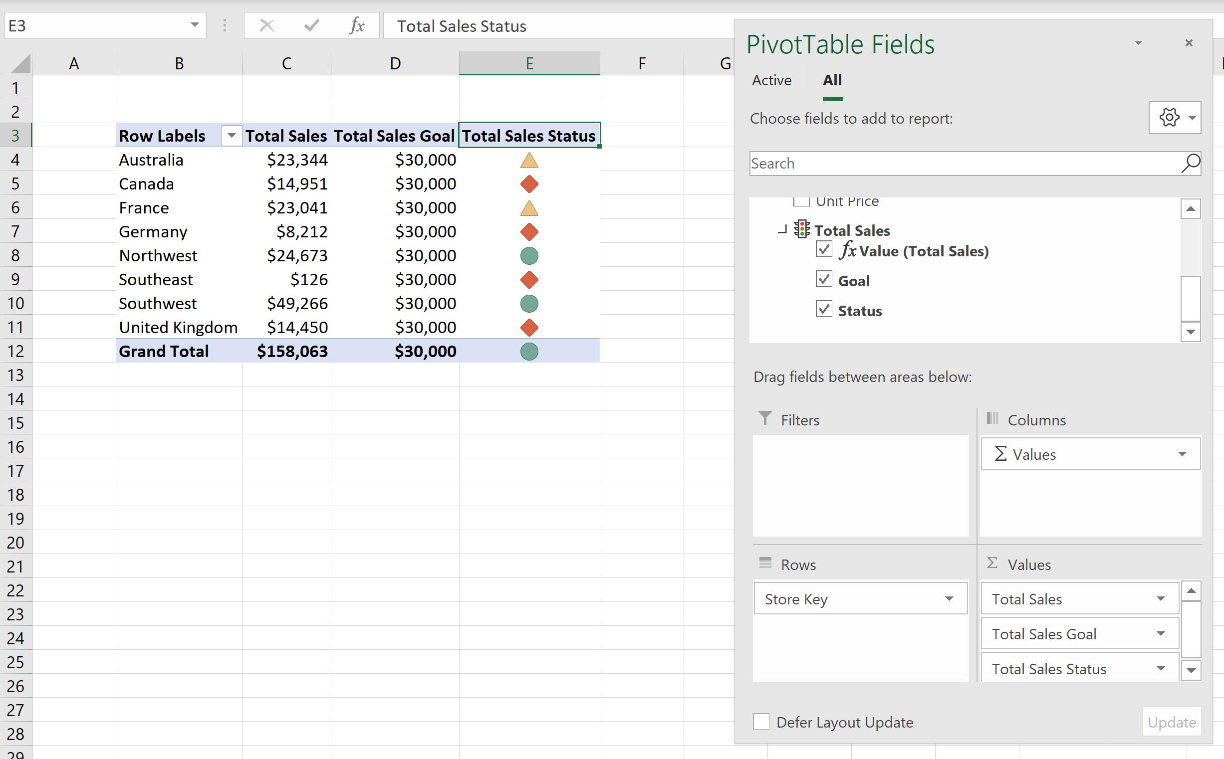
In the ‘PivotTable Fields’ pane, we can see a traffic light icon next to the Total Sales item, and it is expanded so that we can choose to also display the Goal (which is the target value) and Status (which are the coloured icons):
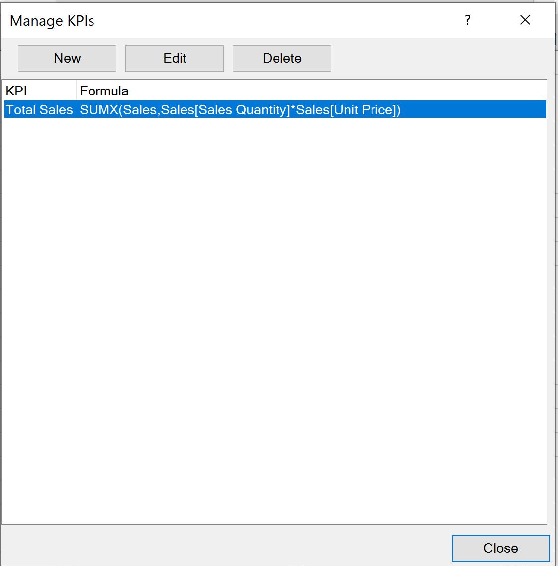
If we wish to modify the KPI, we can navigate back to the ‘Power Pivot’ tab on the Ribbon, click on KPIs -> Manage KPIs…, and choose a KPI we wish to adjust, by clicking Edit:
We can redefine the target value, icon style and status thresholds, then click OK:
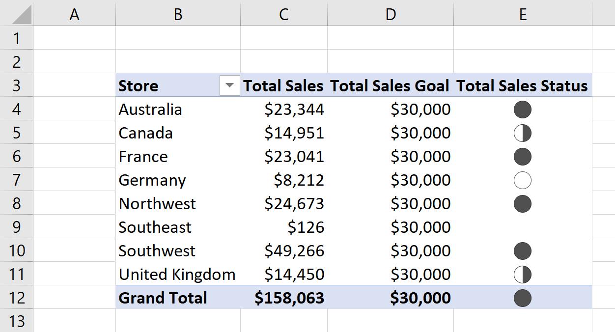
The KPI is now changed:
That’s it for this week!
Stay tuned for our next post on Power Pivot in the Blog section. In the meantime, please remember we have training in Power Pivot which you can find out more about here. If you wish to catch up on past articles in the meantime, you can find all of our Past Power Pivot blogs here.