Power Pivot Principles: Introducing the SUBSTITUTE Function

Welcome back to our Power Pivot blog. Today, we look at the SUBSTITUTE function.

Last week, we looked at the REPLACE function and how it can be used to replace part of a string of text in a column. However, we ran into a problem when we wanted to replace a string of text that existed in different positions in each row. For example, if consider the following dataset:

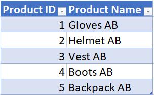
In this scenario we want to replace “AB” with “New”.  Notice that the positions of “AB” in “Gloves AB” and “Vest AB” differ; “AB” is in the eighth character position in “Gloves AB” and is in the sixth character position in “Vest AB”.  In “Gloves AB”, we count each letter as a character position (including blanks), hence why “AB” is in the eighth character position.  When we create the following measure to replace “AB” with “New” using the REPLACE function:

we end up with this result:

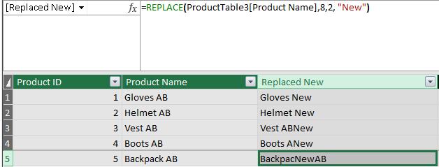
This is because the REPLACE function doesn’t necessarily ‘look’ for “AB”; it just replaces the old text starting from the specified starting character position.

Cue the SUBTITUTE function.

Before we use the SUBSTITUTE function, we must understand how it works.  The SUBSTITUTE function, like the REPLACE function, replaces existing text with new text in text strings in every row in a column.  The SUBSTITUTE function is usually used to create calculated columns.

The SUBSTITUTE function uses the following syntax to operate:

• the <text> parameter is the string of text that contains the characters that we want to substitute; this can also refer to a column that contains text
• the <old_text> parameter is the string of text that we want the function to look for in the text> parameter
• the <new_text> parameter is the text string that is going to replace the <old_text>.
• the <instance_num> is the instance which we want the <old_text> to be replaced by the <next_text> parameter if there are multiple <old_text> strings found.

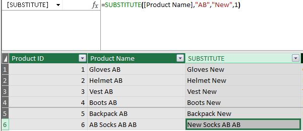
Going back to the dataset mentioned earlier, we can now use the SUBSTITUTE function to create the following measure:

=SUBSTITUTE([Product Name],"AB","New",1)

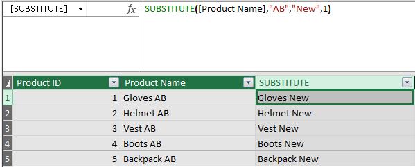
The SUBSTITUTE function has been able to replace all the “AB” text values with “New” without being affected by the different character locations.

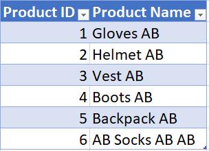
Let’s investigate the <instance_num> parameter. Here, we’ve added another entry to our dataset:

Using the same DAX formula: 

Only the first instance of “AB” has been replaced in position six (6) of our dataset. This is because we specified ‘1’ as our <instance_num>. If we change the <instance_num> to ‘2’ we get:

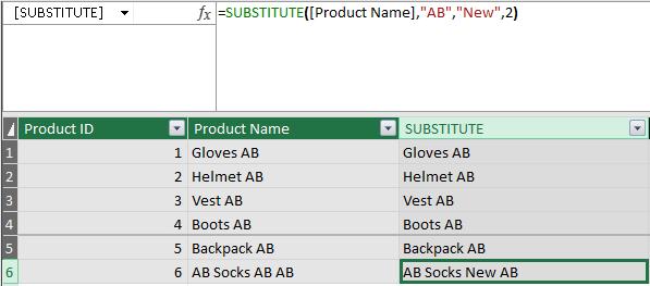
The SUBSTITUTE function now only replaces the second instance of “AB” it finds and ignores the first and last instance. Keep this in mind when using the SUBSTITUTE function: changing the <instance_num> we specify which instance of the <old_text> we want to substitute.

That’s it for this week, tune in next week for more Power Pivot! Until then, happy pivoting!

Stay tuned for our next post on Power Pivot in the Blog section. In the meantime, please remember we have training in Power Pivot which you can find out more about >here. If you wish to catch up on past articles in the meantime, you can find all of our past Power Pivot blogs here.