
Power Pivot Principles: Introducing the NOT Function
28 May 2019
Welcome back to our Power Pivot blog. Today, we introduce the NOT function.
Sometimes we must create custom columns that return with either TRUE or FALSE values. We may also have to create custom columns that have inverse values to another logical column. For example, if we create a custom column with TRUE or FALSE values, we would create another column with the inverse TRUE or FALSE value for each row.
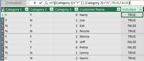
To kick start this example we are going to revisit the custom columns we created for the Conditional Custom Columns Using IF, OR and ‘||’ blog.
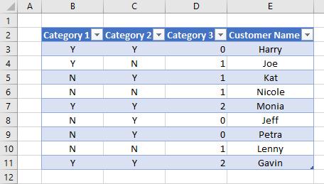
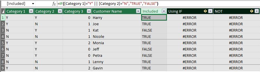
We will use the following Table:
After importing the Table into our data model we are going to create a simple custom column that returns with TRUE when Category 1 is ‘Y’ or Category 2 is ‘N’ (you can read more about using the ‘||’ delimiter here):
=IF([Category 1]="Y" || [Category 2]="N",TRUE,FALSE)
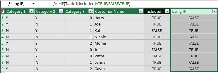
Say we need to create a column with the inverse TRUE or FALSE values, we can use the IF function:
=IF(Table1[Included]=TRUE,FALSE,TRUE)
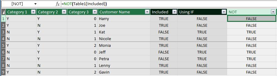
We can also use the NOT function.
The NOT function uses the following syntax:
=NOT([Calculated Column])
With that in mind we can create the following calculated column:
=NOT(Table1[Included])
Rather simple, yes?
One important point to note is that the NOT function requires the [Calculated Column] input to have TRUE or FALSE values. Text values will not be accepted by the NOT function, even if they literally say ‘TRUE’ or ‘FALSE’.
That’s it for this week, tune in next week for more Power Pivot! Until then, happy pivoting!
Stay tuned for our next post on Power Pivot in the Blog section. In the meantime, please remember we have training in Power Pivot which you can find out more about here. If you wish to catch up on past articles in the meantime, you can find all of our Past Power Pivot blogs here.