
Power Pivot Principles: Introducing the DATESINPERIOD Function
30 July 2019
Welcome back to our Power Pivot blog. Today, we show you how the DATESINPERIOD function works.
The DATESINPERIOD function is a time intelligence function, just like the DATESYTD and DATEADD functions. We have covered the DATESYTD and the DATEADD functions previously.
The DATESINPERIOD function uses the following syntax to operate:
DATESINPERIOD( <dates>, <start_date>, <number_of_intervals>, <interval> )
This function returns with a table. This table will contain a column of dates that begins with the <start_date> and continues on with the specified <number_of_intervals>.
The <dates> parameter has to be a column with dates.
The <interval> parameter has to be one of four predefined inputs by Power Pivot: year, quarter, month, day.
This function is commonly used together with the CALCULATE function. You can read more about the CALCULATE function here.
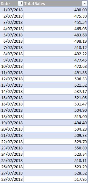
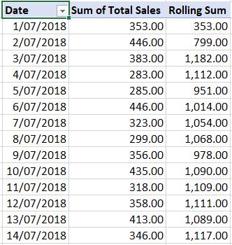
Let’s take a look at a simple example. Imagine we had the following sales data:
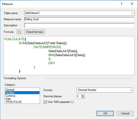
In this example we want to create a rolling sum for every three days. We can use the following measure:
=CALCULATE(
SUM(SaleDataJul1[Total Sales]),
DATESINPERIOD(
SaleDataJul1[Date],
MIN(SaleDataJul1[Date]),
3,
DAY
)
)
This would result in the following PivotTable:
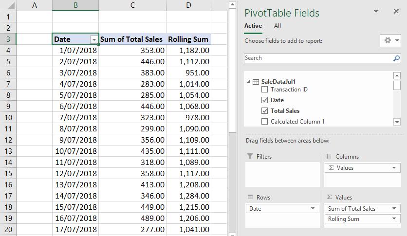
Strangely, the rolling sum seems to be adding up the future dates. This is because we entered ‘3’ as the <number_of_intervals>. Therefore, it looks like positive intervals means that the measure will use future dates. Let’s try ‘-3’:
=CALCULATE(
SUM(SaleDataJul1[Total Sales]),
DATESINPERIOD(
SaleDataJul1[Date],
MIN(SaleDataJul1[Date]),
-3,
DAY
)
)
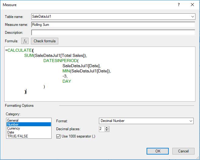
Dragging the new measure into our PivotTable:
Now the measure is adding up sales from the previous dates rather than the future dates. This is all well and good, but having the rolling sum isn’t that useful. What if we changed the SUM function into an AVERAGE function instead?
=CALCULATE(
AVERAGE(SaleDataJul1[Total Sales]),
DATESINPERIOD(
SaleDataJul1[Date],
MIN(SaleDataJul1[Date]),
-3,
DAY
)
)
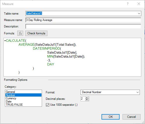
Adding this measure into our PivotTable:
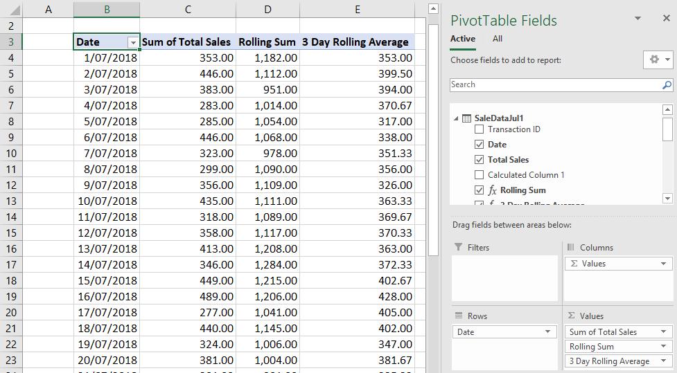
There we have it, a rolling average measure where we can change the number of days / periods we want to include in the average.
That’s it for this week, come back next week for more Power Pivot. Until then happy pivoting!
Stay tuned for our next post on Power Pivot in the Blog section. In the meantime, please remember we have training in Power Pivot which you can find out more about >here. If you wish to catch up on past articles in the meantime, you can find all of our past Power Pivot blogs here.