
Power Pivot Principles: How to Create the CAGR Measure, Part 1
12 March 2019
Welcome back to our Power Pivot blog. Today, we begin a short series on how to create the CAGR measure in Power Pivot.
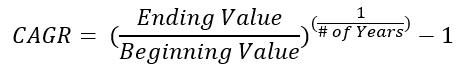
CAGR stands for Compound Annual Growth Rate. It describes the rate at which an investment would have grown over several years if it had grown at the same rate every year on a compounding, rather than simple, basis.
The CAGR metric is calculated using the following formula:
If we were to fit this entire formula into a single measure it may get messy and confusing for other users, so let’s step it out.
We will need to create several measures to calculate the individual pieces the CAGR formula. Of course, this is not the only way to calculate CAGR in Power Pivot, but this is the way we’ve decided to go about it. So, let’s break it down, we will need the following measures to calculate CAGR:
- A measure to retrieve the First Year in the data set
- A measure to retrieve the Last Year in the data set
- A measure to calculate the Number of Years between the First and Last Years in the data set
- A measure to aggregate the total sales in the data set
- A measure to calculate the Sales in the First Year of the data set
- A measure to calculate the Sales in the Last Year of the data set
- Finally, a measure to calculate CAGR.
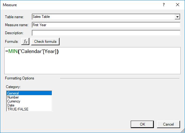
The [First Year] measure is calculated as follows:
=MIN('Calendar'[Year])
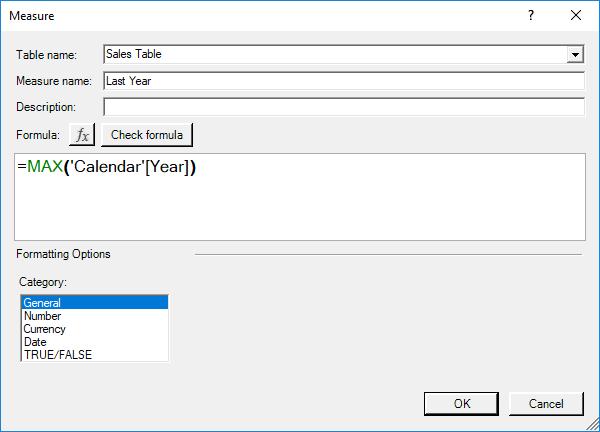
The [Last Year] measure is very similar:
=MAX('Calendar'[Year])
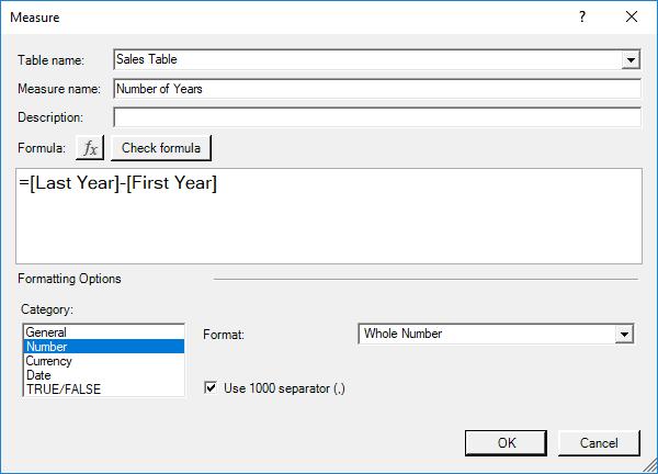
The [Number of Years] measure is simply calculated as the difference between the two years. Unlike calculating dates, you need to resist the urge of adding one to this calculation as there is only one year’s growth between the first year and the next year, etc.
=[Last Year]-[First Year]
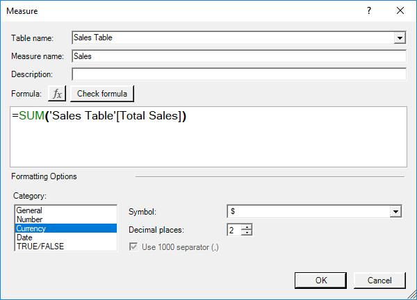
The sales aggregation measure is given by [Sales]:
=SUM('Sales Table'[Total Sales])
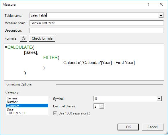
To calculate the [Sales in First Year] measure:
=CALCULATE(
[Sales],
FILTER(
'Calendar','Calendar'[Year]=[First Year]
)
)
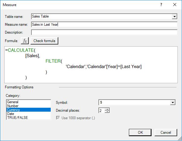
There is therefore no surprise (hopefully!) that [Sales in Last Year] measure is calculated as follows:
=CALCULATE(
[Sales],
FILTER(
'Calendar','Calendar'[Year]=[Last Year]
)
)
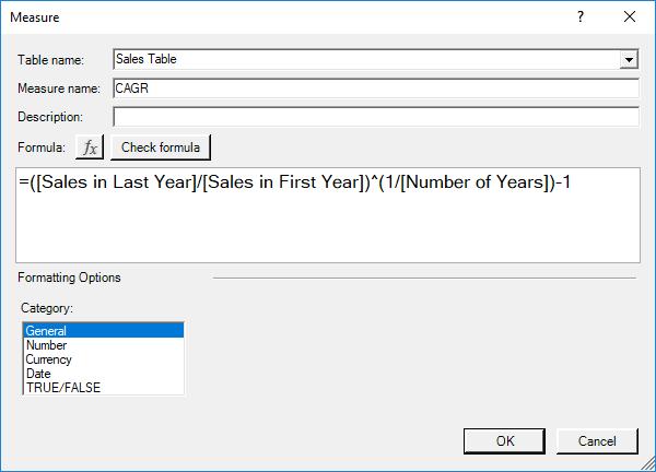
The [CAGR] measure is thus given by:
=([Sales in Last Year]/[Sales in First Year])^(1/[Number of Years])-1
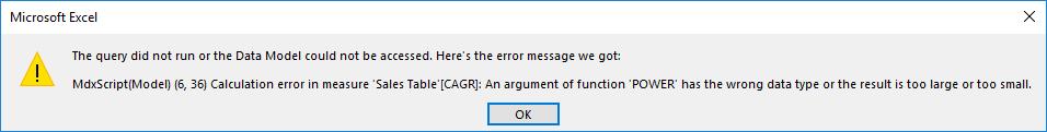
This all seems to make sense. That should be it: let’s create the PivotTable. However, trying to plot our CAGR measure on a PivotTable we get the following message:
Something is not right! Let’s plot the individual measures onto a PivotTable to see if we can figure it out:
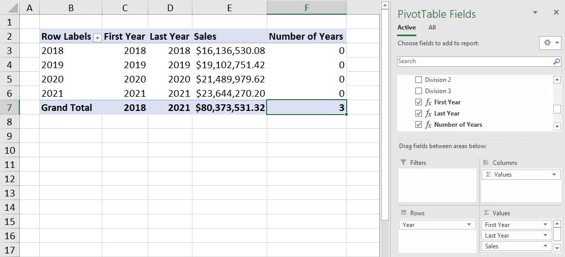
It appears that our [First Year] and [Last Year] measures aren’t working as we intended, hence causing our [Number of Years] measure to return with ‘0’ every year. This causes a division by zero error in our [CAGR] measure.
How do we fix this? We will cover that in next week’s blog.
Until then happy Pivoting, or in this case ‘un-happy Pivoting’!
Stay tuned for our next post on Power Pivot in the Blog section. In the meantime, please remember we have training in Power Pivot which you can find out more about here. If you wish to catch up on past articles in the meantime, you can find all of our Past Power Pivot blogs here.